Change of variables

Last updated

In mathematics, a change of variables is a basic technique used to simplify problems in which the original variables are replaced with functions of other variables. The intent is that when expressed in new variables, the problem may become simpler, or equivalent to a better understood problem.

Contents

Change of variables is an operation that is related to substitution. However these are different operations, as can be seen when considering differentiation (chain rule) or integration (integration by substitution).

A very simple example of a useful variable change can be seen in the problem of finding the roots of the sixth-degree polynomial:

Sixth-degree polynomial equations are generally impossible to solve in terms of radicals (see Abel–Ruffini theorem). This particular equation, however, may be written

(this is a simple case of a polynomial decomposition). Thus the equation may be simplified by defining a new variable . Substituting x by into the polynomial gives

which is just a quadratic equation with the two solutions:

The solutions in terms of the original variable are obtained by substituting x3 back in for u, which gives

Then, assuming that one is interested only in real solutions, the solutions of the original equation are

Simple example

Consider the system of equations

where and are positive integers with . (Source: 1991 AIME)

Solving this normally is not very difficult, but it may get a little tedious. However, we can rewrite the second equation as . Making the substitutions and reduces the system to . Solving this gives and . Back-substituting the first ordered pair gives us , which gives the solution Back-substituting the second ordered pair gives us , which gives no solutions. Hence the solution that solves the system is .

Formal introduction

Let , be smooth manifolds and let be a -diffeomorphism between them, that is: is a times continuously differentiable, bijective map from to with times continuously differentiable inverse from to . Here may be any natural number (or zero), (smooth) or (analytic).

The map is called a regular coordinate transformation or regular variable substitution, where regular refers to the -ness of . Usually one will write to indicate the replacement of the variable by the variable by substituting the value of in for every occurrence of .

Other examples

Coordinate transformation

Some systems can be more easily solved when switching to polar coordinates. Consider for example the equation

This may be a potential energy function for some physical problem. If one does not immediately see a solution, one might try the substitution

given by

Note that if runs outside a -length interval, for example, , the map is no longer bijective. Therefore, should be limited to, for example . Notice how is excluded, for is not bijective in the origin ( can take any value, the point will be mapped to (0, 0)). Then, replacing all occurrences of the original variables by the new expressions prescribed by and using the identity , we get

Now the solutions can be readily found: , so or . Applying the inverse of shows that this is equivalent to while . Indeed, we see that for the function vanishes, except for the origin.

Note that, had we allowed , the origin would also have been a solution, though it is not a solution to the original problem. Here the bijectivity of is crucial. The function is always positive (for ), hence the absolute values.

Differentiation

The chain rule is used to simplify complicated differentiation. For example, consider the problem of calculating the derivative

Let with Then:

Integration

Difficult integrals may often be evaluated by changing variables; this is enabled by the substitution rule and is analogous to the use of the chain rule above. Difficult integrals may also be solved by simplifying the integral using a change of variables given by the corresponding Jacobian matrix and determinant. [1] Using the Jacobian determinant and the corresponding change of variable that it gives is the basis of coordinate systems such as polar, cylindrical, and spherical coordinate systems.

Change of variables formula in terms of Lebesgue measure

The following theorem allows us to relate integrals with respect to Lebesgue measure to an equivalent integral with respect to the pullback measure under a parameterization G. [2] The proof is due to approximations of the Jordan content.

Suppose that is an open subset of and is a diffeomorphism.

  • If is a Lebesgue measurable function on , then is Lebesgue measurable on . If or then .
  • If and is Lebesgue measurable, then is Lebesgue measurable, then .

As a corollary of this theorem, we may compute the Radon–Nikodym derivatives of both the pullback and pushforward measures of under .

Pullback measure and transformation formula

The pullback measure in terms of a transformation is defined as . The change of variables formula for pullback measures is

.

Pushforward measure and transformation formula

The pushforward measure in terms of a transformation , is defined as . The change of variables formula for pushforward measures is

.

As a corollary of the change of variables formula for Lebesgue measure, we have that

  • Radon-Nikodym derivative of the pullback with respect to Lebesgue measure:
  • Radon-Nikodym derivative of the pushforward with respect to Lebesgue measure:

From which we may obtain

  • The change of variables formula for pullback measure:
  • The change of variables formula for pushforward measure:

Differential equations

Variable changes for differentiation and integration are taught in elementary calculus and the steps are rarely carried out in full.

The very broad use of variable changes is apparent when considering differential equations, where the independent variables may be changed using the chain rule or the dependent variables are changed resulting in some differentiation to be carried out. Exotic changes, such as the mingling of dependent and independent variables in point and contact transformations, can be very complicated but allow much freedom.

Very often, a general form for a change is substituted into a problem and parameters picked along the way to best simplify the problem.

Scaling and shifting

Probably the simplest change is the scaling and shifting of variables, that is replacing them with new variables that are "stretched" and "moved" by constant amounts. This is very common in practical applications to get physical parameters out of problems. For an nth order derivative, the change simply results in

where

This may be shown readily through the chain rule and linearity of differentiation. This change is very common in practical applications to get physical parameters out of problems, for example, the boundary value problem

describes parallel fluid flow between flat solid walls separated by a distance δ; μ is the viscosity and the pressure gradient, both constants. By scaling the variables the problem becomes

where

Scaling is useful for many reasons. It simplifies analysis both by reducing the number of parameters and by simply making the problem neater. Proper scaling may normalize variables, that is make them have a sensible unitless range such as 0 to 1. Finally, if a problem mandates numeric solution, the fewer the parameters the fewer the number of computations.

Momentum vs. velocity

Consider a system of equations

for a given function . The mass can be eliminated by the (trivial) substitution . Clearly this is a bijective map from to . Under the substitution the system becomes

Lagrangian mechanics

Given a force field , Newton's equations of motion are

Lagrange examined how these equations of motion change under an arbitrary substitution of variables ,

He found that the equations

are equivalent to Newton's equations for the function , where T is the kinetic, and V the potential energy.

In fact, when the substitution is chosen well (exploiting for example symmetries and constraints of the system) these equations are much easier to solve than Newton's equations in Cartesian coordinates.

See also

Related Research Articles

<span class="mw-page-title-main">Polar coordinate system</span> Coordinates comprising a distance and an angle

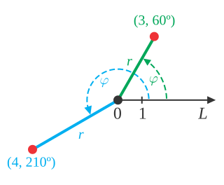
In mathematics, the polar coordinate system is a two-dimensional coordinate system in which each point on a plane is determined by a distance from a reference point and an angle from a reference direction. The reference point is called the pole, and the ray from the pole in the reference direction is the polar axis. The distance from the pole is called the radial coordinate, radial distance or simply radius, and the angle is called the angular coordinate, polar angle, or azimuth. Angles in polar notation are generally expressed in either degrees or radians.

<span class="mw-page-title-main">Navier–Stokes equations</span> Equations describing the motion of viscous fluid substances

The Navier–Stokes equations are partial differential equations which describe the motion of viscous fluid substances. They were named after French engineer and physicist Claude-Louis Navier and the Irish physicist and mathematician George Gabriel Stokes. They were developed over several decades of progressively building the theories, from 1822 (Navier) to 1842–1850 (Stokes).
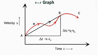
<span class="mw-page-title-main">Potential flow</span> Velocity field as the gradient of a scalar function

In fluid dynamics, potential flow or irrotational flow refers to a description of a fluid flow with no vorticity in it. Such a description typically arises in the limit of vanishing viscosity, i.e., for an inviscid fluid and with no vorticity present in the flow.

<span class="mw-page-title-main">Tautochrone curve</span> Curve for which the time to roll to the end is equal for all starting points

A tautochrone curve or isochrone curve is the curve for which the time taken by an object sliding without friction in uniform gravity to its lowest point is independent of its starting point on the curve. The curve is a cycloid, and the time is equal to π times the square root of the radius over the acceleration of gravity. The tautochrone curve is related to the brachistochrone curve, which is also a cycloid.

In calculus, integration by substitution, also known as u-substitution, reverse chain rule or change of variables, is a method for evaluating integrals and antiderivatives. It is the counterpart to the chain rule for differentiation, and can loosely be thought of as using the chain rule "backwards."

<span class="mw-page-title-main">Jensen's inequality</span> Theorem of convex functions

In mathematics, Jensen's inequality, named after the Danish mathematician Johan Jensen, relates the value of a convex function of an integral to the integral of the convex function. It was proved by Jensen in 1906, building on an earlier proof of the same inequality for doubly-differentiable functions by Otto Hölder in 1889. Given its generality, the inequality appears in many forms depending on the context, some of which are presented below. In its simplest form the inequality states that the convex transformation of a mean is less than or equal to the mean applied after convex transformation; it is a simple corollary that the opposite is true of concave transformations.

Linear elasticity is a mathematical model of how solid objects deform and become internally stressed due to prescribed loading conditions. It is a simplification of the more general nonlinear theory of elasticity and a branch of continuum mechanics.

The primitive equations are a set of nonlinear partial differential equations that are used to approximate global atmospheric flow and are used in most atmospheric models. They consist of three main sets of balance equations:

  1. A continuity equation: Representing the conservation of mass.
  2. Conservation of momentum: Consisting of a form of the Navier–Stokes equations that describe hydrodynamical flow on the surface of a sphere under the assumption that vertical motion is much smaller than horizontal motion (hydrostasis) and that the fluid layer depth is small compared to the radius of the sphere
  3. A thermal energy equation: Relating the overall temperature of the system to heat sources and sinks

In mathematics, the symmetry of second derivatives refers to the possibility of interchanging the order of taking partial derivatives of a function

<span class="mw-page-title-main">Particle in a spherically symmetric potential</span> Quantum mechanical model

In quantum mechanics, a particle in a spherically symmetric potential is a system with a potential that depends only on the distance between the particle and a center. A particle in a spherically symmetric potential can be used as an approximation, for example, of the electron in a hydrogen atom or of the formation of chemical bonds.

In probability theory, the Borel–Kolmogorov paradox is a paradox relating to conditional probability with respect to an event of probability zero. It is named after Émile Borel and Andrey Kolmogorov.

<span class="mw-page-title-main">Propagator</span> Function in quantum field theory showing probability amplitudes of moving particles

In quantum mechanics and quantum field theory, the propagator is a function that specifies the probability amplitude for a particle to travel from one place to another in a given period of time, or to travel with a certain energy and momentum. In Feynman diagrams, which serve to calculate the rate of collisions in quantum field theory, virtual particles contribute their propagator to the rate of the scattering event described by the respective diagram. Propagators may also be viewed as the inverse of the wave operator appropriate to the particle, and are, therefore, often called (causal) Green's functions.

In calculus, the Leibniz integral rule for differentiation under the integral sign states that for an integral of the form

In mathematics, subharmonic and superharmonic functions are important classes of functions used extensively in partial differential equations, complex analysis and potential theory.

<span class="mw-page-title-main">Hopf bifurcation</span> Critical point where a periodic solution arises

In the mathematical theory of bifurcations, a Hopfbifurcation is a critical point where, as a parameter changes, a system's stability switches and a periodic solution arises. More accurately, it is a local bifurcation in which a fixed point of a dynamical system loses stability, as a pair of complex conjugate eigenvalues—of the linearization around the fixed point—crosses the complex plane imaginary axis as a parameter crosses a threshold value. Under reasonably generic assumptions about the dynamical system, the fixed point becomes a small-amplitude limit cycle as the parameter changes.

A theoretical motivation for general relativity, including the motivation for the geodesic equation and the Einstein field equation, can be obtained from special relativity by examining the dynamics of particles in circular orbits about the Earth. A key advantage in examining circular orbits is that it is possible to know the solution of the Einstein Field Equation a priori. This provides a means to inform and verify the formalism.

<span class="mw-page-title-main">Radiative transfer equation and diffusion theory for photon transport in biological tissue</span>

Photon transport in biological tissue can be equivalently modeled numerically with Monte Carlo simulations or analytically by the radiative transfer equation (RTE). However, the RTE is difficult to solve without introducing approximations. A common approximation summarized here is the diffusion approximation. Overall, solutions to the diffusion equation for photon transport are more computationally efficient, but less accurate than Monte Carlo simulations.

In mathematics, the spectral theory of ordinary differential equations is the part of spectral theory concerned with the determination of the spectrum and eigenfunction expansion associated with a linear ordinary differential equation. In his dissertation, Hermann Weyl generalized the classical Sturm–Liouville theory on a finite closed interval to second order differential operators with singularities at the endpoints of the interval, possibly semi-infinite or infinite. Unlike the classical case, the spectrum may no longer consist of just a countable set of eigenvalues, but may also contain a continuous part. In this case the eigenfunction expansion involves an integral over the continuous part with respect to a spectral measure, given by the Titchmarsh–Kodaira formula. The theory was put in its final simplified form for singular differential equations of even degree by Kodaira and others, using von Neumann's spectral theorem. It has had important applications in quantum mechanics, operator theory and harmonic analysis on semisimple Lie groups.

<span class="mw-page-title-main">Mild-slope equation</span> Physics phenomenon and formula

In fluid dynamics, the mild-slope equation describes the combined effects of diffraction and refraction for water waves propagating over bathymetry and due to lateral boundaries—like breakwaters and coastlines. It is an approximate model, deriving its name from being originally developed for wave propagation over mild slopes of the sea floor. The mild-slope equation is often used in coastal engineering to compute the wave-field changes near harbours and coasts.

In mathematics, singular integral operators of convolution type are the singular integral operators that arise on Rn and Tn through convolution by distributions; equivalently they are the singular integral operators that commute with translations. The classical examples in harmonic analysis are the harmonic conjugation operator on the circle, the Hilbert transform on the circle and the real line, the Beurling transform in the complex plane and the Riesz transforms in Euclidean space. The continuity of these operators on L2 is evident because the Fourier transform converts them into multiplication operators. Continuity on Lp spaces was first established by Marcel Riesz. The classical techniques include the use of Poisson integrals, interpolation theory and the Hardy–Littlewood maximal function. For more general operators, fundamental new techniques, introduced by Alberto Calderón and Antoni Zygmund in 1952, were developed by a number of authors to give general criteria for continuity on Lp spaces. This article explains the theory for the classical operators and sketches the subsequent general theory.

References

  1. Kaplan, Wilfred (1973). "Change of Variables in Integrals". Advanced Calculus (Second ed.). Reading: Addison-Wesley. pp. 269–275.
  2. Folland, G. B. (1999). Real analysis : modern techniques and their applications (2nd ed.). New York: Wiley. pp. 74–75. ISBN   0-471-31716-0. OCLC   39849337.