Discrete calculus

This article is about the discrete version of calculus. It is not to be confused with Discretization in calculus.

Discrete calculus or the calculus of discrete functions, is the mathematical study of incremental change, in the same way that geometry is the study of shape and algebra is the study of generalizations of arithmetic operations. The word calculus is a Latin word, meaning originally "small pebble"; as such pebbles were used for calculation, the meaning of the word has evolved and today usually means a method of computation. Meanwhile, calculus , originally called infinitesimal calculus or "the calculus of infinitesimals", is the study of continuous change.

Discrete calculus has two entry points, differential calculus and integral calculus. Differential calculus concerns incremental rates of change and the slopes of piece-wise linear curves. Integral calculus concerns accumulation of quantities and the areas under piece-wise constant curves. These two points of view are related to each other by the fundamental theorem of discrete calculus.

The study of the concepts of change starts with their discrete form. The development is dependent on a parameter, the increment ${\displaystyle \Delta x}$ of the independent variable. If we so choose, we can make the increment smaller and smaller and find the continuous counterparts of these concepts as limits. Informally, the limit of discrete calculus as ${\displaystyle \Delta x\to 0}$ is infinitesimal calculus. Even though it serves as a discrete underpinning of calculus, the main value of discrete calculus is in applications.

Two initial constructions

Discrete differential calculus is the study of the definition, properties, and applications of the difference quotient of a function. The process of finding the difference quotient is called differentiation. Given a function defined at several points of the real line, the difference quotient at that point is a way of encoding the small-scale (i.e., from the point to the next) behavior of the function. By finding the difference quotient of a function at every pair of consecutive points in its domain, it is possible to produce a new function, called the difference quotient function or just the difference quotient of the original function. In formal terms, the difference quotient is a linear operator which takes a function as its input and produces a second function as its output. This is more abstract than many of the processes studied in elementary algebra, where functions usually input a number and output another number. For example, if the doubling function is given the input three, then it outputs six, and if the squaring function is given the input three, then it outputs nine. The derivative, however, can take the squaring function as an input. This means that the derivative takes all the information of the squaring function—such as that two is sent to four, three is sent to nine, four is sent to sixteen, and so on—and uses this information to produce another function. The function produced by differentiating the squaring function turns out to be something close to the doubling function.

Suppose the functions are defined at points separated by an increment ${\displaystyle \Delta x=h>0}$:

${\displaystyle a,a+h,a+2h,\ldots ,a+nh,\ldots }$

The "doubling function" may be denoted by ${\displaystyle g(x)=2x}$ and the "squaring function" by ${\displaystyle f(x)=x^{2}}$. The "difference quotient" is the rate of change of the function over one of the intervals ${\displaystyle [x,x+h]}$ defined by the formula:

${\displaystyle {\frac {f(x+h)-f(x)}{h}}.}$

It takes the function ${\displaystyle f}$ as an input, that is all the information—such as that two is sent to four, three is sent to nine, four is sent to sixteen, and so on—and uses this information to output another function, the function ${\displaystyle g(x)=2x+h}$, as will turn out. As a matter of convenience, the new function may defined at the middle points of the above intervals:

${\displaystyle a+h/2,a+h+h/2,a+2h+h/2,...,a+nh+h/2,...}$

As the rate of change is that for the whole interval ${\displaystyle [x,x+h]}$, any point within it can be used as such a reference or, even better, the whole interval which makes the difference quotient a ${\displaystyle 1}$-cochain.

The most common notation for the difference quotient is:

${\displaystyle {\frac {\Delta f}{\Delta x}}(x+h/2)={\frac {f(x+h)-f(x)}{h}}.}$

If the input of the function represents time, then the difference quotient represents change with respect to time. For example, if ${\displaystyle f}$ is a function that takes a time as input and gives the position of a ball at that time as output, then the difference quotient of ${\displaystyle f}$ is how the position is changing in time, that is, it is the velocity of the ball.

If a function is linear (that is, if the points of the graph of the function lie on a straight line), then the function can be written as ${\displaystyle y=mx+b}$, where ${\displaystyle x}$ is the independent variable, ${\displaystyle y}$ is the dependent variable, ${\displaystyle b}$ is the ${\displaystyle y}$-intercept, and:

${\displaystyle m={\frac {\text{rise}}{\text{run}}}={\frac {{\text{change in }}y}{{\text{change in }}x}}={\frac {\Delta y}{\Delta x}}.}$

Slope: ${\displaystyle m={\frac {\Delta y}{\Delta x}}=\tan(\theta )}$

This gives an exact value for the slope of a straight line.

If the function is not linear, however, then the change in ${\displaystyle y}$ divided by the change in ${\displaystyle x}$ varies. The difference quotient give an exact meaning to the notion of change in output with respect to change in input. To be concrete, let ${\displaystyle f}$ be a function, and fix a point ${\displaystyle x}$ in the domain of ${\displaystyle f}$. ${\displaystyle (x,f(x))}$ is a point on the graph of the function. If ${\displaystyle h}$ is the increment of ${\displaystyle x}$, then ${\displaystyle x+h}$ is the next value of ${\displaystyle x}$. Therefore, ${\displaystyle (x+h,f(x+h))}$ is the increment of ${\displaystyle (x,f(x))}$. The slope of the line between these two points is

${\displaystyle m={\frac {f(x+h)-f(x)}{(x+h)-x}}={\frac {f(x+h)-f(x)}{h}}.}$

So ${\displaystyle m}$ is the slope of the line between ${\displaystyle (x,f(x))}$ and ${\displaystyle (x+h,f(x+h))}$.

Here is a particular example, the difference quotient of the squaring function. Let ${\displaystyle f(x)=x^{2}}$ be the squaring function. Then:

${\displaystyle {\begin{aligned}{\frac {\Delta f}{\Delta x}}(x)&={(x+h)^{2}-x^{2} \over {h}}\\&={x^{2}+2hx+h^{2}-x^{2} \over {h}}\\&={2hx+h^{2} \over {h}}\\&=2x+h.\end{aligned}}}$

The difference quotient of the difference quotient is called the second difference quotient and it is defined at

${\displaystyle a+h,a+2h,a+3h,\ldots ,a+nh,\ldots }$

and so on.

Discrete integral calculus is the study of the definitions, properties, and applications of the Riemann sums. The process of finding the value of a sum is called integration. In technical language, integral calculus studies a certain linear operator.

The Riemann sum inputs a function and outputs a function, which gives the algebraic sum of areas between the part of the graph of the input and the x-axis.

A motivating example is the distances traveled in a given time.

${\displaystyle {\text{distance}}={\text{speed}}\cdot {\text{time}}}$

If the speed is constant, only multiplication is needed, but if the speed changes, we evaluate the distance traveled by breaking up the time into many short intervals of time, then multiplying the time elapsed in each interval by one of the speeds in that interval, and then taking the sum (a Riemann sum) of the distance traveled in each interval.

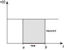
Constant velocity

The Riemann sum is measuring the total area of the bars, defined by ${\displaystyle f}$, between two points (here ${\displaystyle a}$ and ${\displaystyle b}$).

When velocity is constant, the total distance traveled over the given time interval can be computed by multiplying velocity and time. For example, travelling a steady 50 mph for 3 hours results in a total distance of 150 miles. In the diagram on the left, when constant velocity and time are graphed, these two values form a rectangle with height equal to the velocity and width equal to the time elapsed. Therefore, the product of velocity and time also calculates the rectangular area under the (constant) velocity curve. This connection between the area under a curve and distance traveled can be extended to any irregularly shaped region exhibiting an incrementally varying velocity over a given time period. If the bars in the diagram on the right represents speed as it varies from an interval to the next, the distance traveled (between the times represented by ${\displaystyle a}$ and ${\displaystyle b}$) is the area of the shaded region ${\displaystyle s}$.

So, the interval between ${\displaystyle a}$ and ${\displaystyle b}$ is divided into a number of equal segments, the length of each segment represented by the symbol ${\displaystyle \Delta x}$. For each small segment, we have one value of the function ${\displaystyle f(x)}$. Call that value ${\displaystyle v}$. Then the area of the rectangle with base ${\displaystyle \Delta x}$ and height ${\displaystyle v}$ gives the distance (time ${\displaystyle \Delta x}$ multiplied by speed ${\displaystyle v}$) traveled in that segment. Associated with each segment is the value of the function above it, ${\displaystyle f(x)=v}$. The sum of all such rectangles gives the area between the axis and the piece-wise constant curve, which is the total distance traveled.

Suppose a function is defined at the mid-points of the intervals of equal length ${\displaystyle \Delta x=h>0}$:

${\displaystyle a+h/2,a+h+h/2,a+2h+h/2,\ldots ,a+nh-h/2,\ldots }$

Then the Riemann sum from ${\displaystyle a}$ to ${\displaystyle b=a+nh}$ in sigma notation is:

${\displaystyle \sum _{i=1}^{n}f(a+ih)\,\Delta x.}$

As this computation is carried out for each ${\displaystyle n}$, the new function is defined at the points:

${\displaystyle a,a+h,a+2h,\ldots ,a+nh,\ldots }$

The fundamental theorem of calculus states that differentiation and integration are inverse operations. More precisely, it relates the difference quotients to the Riemann sums. It can also be interpreted as a precise statement of the fact that differentiation is the inverse of integration.

The fundamental theorem of calculus: If a function ${\displaystyle f}$ is defined on a partition of the interval ${\displaystyle [a,b]}$, ${\displaystyle b=a+nh}$, and if ${\displaystyle F}$ is a function whose difference quotient is ${\displaystyle f}$, then we have:

${\displaystyle \sum _{i=0}^{n-1}f(a+ih+h/2)\,\Delta x=F(b)-F(a).}$

Furthermore, for every ${\textstyle m=0,1,2,\ldots ,n-1}$, we have:

${\displaystyle {\frac {\Delta }{\Delta x}}\sum _{i=0}^{m}f(a+ih+h/2)\,\Delta x=f(a+mh+h/2).}$

This is also a prototype solution of a difference equation. Difference equations relate an unknown function to its difference or difference quotient, and are ubiquitous in the sciences.

History

The early history of discrete calculus is the history of calculus. Such basic ideas as the difference quotients and the Riemann sums appear implicitly or explicitly in definitions and proofs. After the limit is taken, however, they are never to be seen again. However, the Kirchhoff's voltage law (1847) can be expressed in terms of the one-dimensional discrete exterior derivative.

During the 20th century discrete calculus remains interlinked with infinitesimal calculus especially differential forms but also starts to draw from algebraic topology as both develop. The main contributions come from the following individuals: ^[1]

• Henri Poincaré: triangulations (barycentric subdivision, dual triangulation), Poincare lemma, the first proof of the general Stokes Theorem, and a lot more
• L. E. J. Brouwer: simplicial approximation theorem
• Élie Cartan, Georges de Rham: the notion of differential form, the exterior derivative as a coordinate-independent linear operator, exactness/closedness of forms
• Emmy Noether, Heinz Hopf, Leopold Vietoris, Walther Mayer: modules of chains, the boundary operator, chain complexes
• J. W. Alexander, Solomon Lefschetz, Lev Pontryagin, Andrey Kolmogorov, Norman Steenrod, Eduard Čech: the early cochain notions
• Hermann Weyl: the Kirchhoff laws stated in terms of the boundary and the coboundary operators
• W. V. D. Hodge: the Hodge star operator, the Hodge decomposition
• Samuel Eilenberg, Saunders Mac Lane, Norman Steenrod, J.H.C. Whitehead: the rigorous development of homology and cohomology theory including chain and cochain complexes, the cup product
• Hassler Whitney: cochains as integrands

The recent development of discrete calculus, starting with Whitney, has been driven by the needs of applied modeling. ^{[2] [3] [4]}

Applications

Discrete calculus is used for modeling either directly or indirectly as a discretization of infinitesimal calculus in every branch of the physical sciences, actuarial science, computer science, statistics, engineering, economics, business, medicine, demography, and in other fields wherever a problem can be mathematically modeled. It allows one to go from (non-constant) rates of change to the total change or vice versa, and many times in studying a problem we know one and are trying to find the other.

Physics makes particular use of calculus; all discrete concepts in classical mechanics and electromagnetism are related through discrete calculus. The mass of an object of known density that varies incrementally, the moment of inertia of such objects, as well as the total energy of an object within a discrete conservative field can be found by the use of discrete calculus. An example of the use of discrete calculus in mechanics is Newton's second law of motion: historically stated it expressly uses the term "change of motion" which implies the difference quotient saying The change of momentum of a body is equal to the resultant force acting on the body and is in the same direction. Commonly expressed today as Force = Mass × Acceleration, it invokes discrete calculus when the change is incremental because acceleration is the difference quotient of velocity with respect to time or second difference quotient of the spatial position. Starting from knowing how an object is accelerating, we use the Riemann sums to derive its path.

Maxwell's theory of electromagnetism and Einstein's theory of general relativity have been expressed in the language of discrete calculus.

Chemistry uses calculus in determining reaction rates and radioactive decay (exponential decay).

In biology, population dynamics starts with reproduction and death rates to model population changes (population modeling).

In engineering, difference equations are used to plot a course of a spacecraft within zero gravity environments, to model heat transfer, diffusion, and wave propagation.

The discrete analogue of Green's theorem is applied in an instrument known as a planimeter, which is used to calculate the area of a flat surface on a drawing. For example, it can be used to calculate the amount of area taken up by an irregularly shaped flower bed or swimming pool when designing the layout of a piece of property. It can be used to efficiently calculate sums of rectangular domains in images, to rapidly extract features and detect object; another algorithm that could be used is the summed area table.

In the realm of medicine, calculus can be used to find the optimal branching angle of a blood vessel so as to maximize flow. From the decay laws for a particular drug's elimination from the body, it is used to derive dosing laws. In nuclear medicine, it is used to build models of radiation transport in targeted tumor therapies.

In economics, calculus allows for the determination of maximal profit by calculating both marginal cost and marginal revenue, as well as modeling of markets. ^[5]

In signal processing and machine learning, discrete calculus allows for appropriate definitions of operators (e.g., convolution), level set optimization and other key functions for neural network analysis on graph structures. ^[3]

Discrete calculus can be used in conjunction with other mathematical disciplines. For example, it can be used in probability theory to determine the probability of a discrete random variable from an assumed density function.

Calculus of differences and sums

Suppose a function (a ${\displaystyle 0}$-cochain) ${\displaystyle f}$ is defined at points separated by an increment ${\displaystyle \Delta x=h>0}$:

${\displaystyle a,a+h,a+2h,\ldots ,a+nh,\ldots }$

The difference (or the exterior derivative, or the coboundary operator) of the function is given by:

${\displaystyle {\big (}\Delta f{\big )}{\big (}[x,x+h]{\big )}=f(x+h)-f(x).}$

It is defined at each of the above intervals; it is a ${\displaystyle 1}$-cochain.

Suppose a ${\displaystyle 1}$-cochain ${\displaystyle g}$ is defined at each of the above intervals. Then its sum is a function (a ${\displaystyle 0}$-cochain) defined at each of the points by:

${\displaystyle \left(\sum g\right)\!(a+nh)=\sum _{i=1}^{n}g{\big (}[a+(i-1)h,a+ih]{\big )}.}$

These are their properties:

• Constant rule: If ${\displaystyle c}$ is a constant, then

${\displaystyle \Delta c=0}$

• Linearity : if ${\displaystyle a}$ and ${\displaystyle b}$ are constants,

${\displaystyle \Delta (af+bg)=a\,\Delta f+b\,\Delta g,\quad \sum (af+bg)=a\,\sum f+b\,\sum g}$

• Product rule :

${\displaystyle \Delta (fg)=f\,\Delta g+g\,\Delta f+\Delta f\,\Delta g}$

• Fundamental theorem of calculus I:

${\displaystyle \left(\sum \Delta f\right)\!(a+nh)=f(a+nh)-f(a)}$

• Fundamental theorem of calculus II:

${\displaystyle \Delta \!\left(\sum g\right)=g}$

The definitions are applied to graphs as follows. If a function (a ${\displaystyle 0}$-cochain) ${\displaystyle f}$ is defined at the nodes of a graph:

${\displaystyle a,b,c,\ldots }$

then its exterior derivative (or the differential) is the difference, i.e., the following function defined on the edges of the graph (${\displaystyle 1}$-cochain):

${\displaystyle \left(df\right)\!{\big (}[a,b]{\big )}=f(b)-f(a).}$

If ${\displaystyle g}$ is a ${\displaystyle 1}$-cochain, then its integral over a sequence of edges ${\displaystyle \sigma }$ of the graph is the sum of its values over all edges of ${\displaystyle \sigma }$ ("path integral"):

${\displaystyle \int _{\sigma }g=\sum _{\sigma }g{\big (}[a,b]{\big )}.}$

These are the properties:

• Constant rule: If ${\displaystyle c}$ is a constant, then

${\displaystyle dc=0}$

• Linearity: if ${\displaystyle a}$ and ${\displaystyle b}$ are constants,

${\displaystyle d(af+bg)=a\,df+b\,dg,\quad \int _{\sigma }(af+bg)=a\,\int _{\sigma }f+b\,\int _{\sigma }g}$

• Product rule:

${\displaystyle d(fg)=f\,dg+g\,df+df\,dg}$

• Fundamental theorem of calculus I: if a ${\displaystyle 1}$-chain ${\displaystyle \sigma }$ consists of the edges ${\displaystyle [a_{0},a_{1}],[a_{1},a_{2}],...,[a_{n-1},a_{n}]}$, then for any ${\displaystyle 0}$-cochain ${\displaystyle f}$

${\displaystyle \int _{\sigma }df=f(a_{n})-f(a_{0})}$

• Fundamental theorem of calculus II: if the graph is a tree, ${\displaystyle g}$ is a ${\displaystyle 1}$-cochain, and a function (${\displaystyle 0}$-cochain) is defined on the nodes of the graph by

${\displaystyle f(x)=\int _{\sigma }g}$

where a ${\displaystyle 1}$-chain ${\displaystyle \sigma }$ consists of ${\displaystyle [a_{0},a_{1}],[a_{1},a_{2}],...,[a_{n-1},x]}$ for some fixed ${\displaystyle a_{0}}$, then

${\displaystyle df=g}$

See references. ^{[6] [7] [8] [9] [3] [10]}

Chains of simplices and cubes

A simplicial complex.

A simplicial complex ${\displaystyle S}$ is a set of simplices that satisfies the following conditions:

1. Every face of a simplex from ${\displaystyle S}$ is also in ${\displaystyle S}$.

2. The non-empty intersection of any two simplices ${\displaystyle \sigma _{1},\sigma _{2}\in S}$ is a face of both ${\displaystyle \sigma _{1}}$ and ${\displaystyle \sigma _{2}}$.

The boundary of a boundary of a 2-simplex (left) and the boundary of a 1-chain (right) are taken. Both are 0, being sums in which both the positive and negative of a 0-simplex occur once. The boundary of a boundary is always 0. A nontrivial cycle is something that closes up like the boundary of a simplex, in that its boundary sums to 0, but which isn't actually the boundary of a simplex or chain.

By definition, an orientation of a k-simplex is given by an ordering of the vertices, written as ${\displaystyle (v_{0},...,v_{k})}$, with the rule that two orderings define the same orientation if and only if they differ by an even permutation. Thus every simplex has exactly two orientations, and switching the order of two vertices changes an orientation to the opposite orientation. For example, choosing an orientation of a 1-simplex amounts to choosing one of the two possible directions, and choosing an orientation of a 2-simplex amounts to choosing what "counterclockwise" should mean.

Let ${\displaystyle S}$ be a simplicial complex. A simplicial k-chain is a finite formal sum

${\displaystyle \sum _{i=1}^{N}c_{i}\sigma _{i},\,}$

where each c_i is an integer and σ_i is an oriented k-simplex. In this definition, we declare that each oriented simplex is equal to the negative of the simplex with the opposite orientation. For example,

${\displaystyle (v_{0},v_{1})=-(v_{1},v_{0}).}$

The vector space of k-chains on ${\displaystyle S}$ is written ${\displaystyle C_{k}}$. It has a basis in one-to-one correspondence with the set of k-simplices in ${\displaystyle S}$. To define a basis explicitly, one has to choose an orientation of each simplex. One standard way to do this is to choose an ordering of all the vertices and give each simplex the orientation corresponding to the induced ordering of its vertices.

Let ${\displaystyle \sigma =(v_{0},...,v_{k})}$ be an oriented k-simplex, viewed as a basis element of ${\displaystyle C_{k}}$. The boundary operator

${\displaystyle \partial _{k}:C_{k}\rightarrow C_{k-1}}$

is the linear operator defined by:

${\displaystyle \partial _{k}(\sigma )=\sum _{i=0}^{k}(-1)^{i}(v_{0},\dots ,{\widehat {v_{i}}},\dots ,v_{k}),}$

where the oriented simplex

${\displaystyle (v_{0},\dots ,{\widehat {v_{i}}},\dots ,v_{k})}$

is the ${\displaystyle i}$th face of ${\displaystyle \sigma }$, obtained by deleting its ${\displaystyle i}$th vertex.

In ${\displaystyle C_{k}}$, elements of the subgroup

${\displaystyle Z_{k}=\ker \partial _{k}}$

are referred to as cycles, and the subgroup

${\displaystyle B_{k}=\operatorname {im} \partial _{k+1}}$

is said to consist of boundaries.

A direct computation shows that ${\displaystyle \partial ^{2}=0}$. In geometric terms, this says that the boundary of anything has no boundary. Equivalently, the vector spaces ${\displaystyle (C_{k},\partial _{k})}$ form a chain complex. Another equivalent statement is that ${\displaystyle B_{k}}$ is contained in ${\displaystyle Z_{k}}$.

A cubical complex is a set composed of points, line segments, squares, cubes, and their n-dimensional counterparts. They are used analogously to simplices to form complexes. An elementary interval is a subset ${\displaystyle I\subset \mathbf {R} }$ of the form

${\displaystyle I=[\ell ,\ell +1]\quad {\text{or}}\quad I=[\ell ,\ell ]}$

for some ${\displaystyle \ell \in \mathbf {Z} }$. An elementary cube${\displaystyle Q}$ is the finite product of elementary intervals, i.e.

${\displaystyle Q=I_{1}\times I_{2}\times \cdots \times I_{d}\subset \mathbf {R} ^{d}}$

where ${\displaystyle I_{1},I_{2},\ldots ,I_{d}}$ are elementary intervals. Equivalently, an elementary cube is any translate of a unit cube ${\displaystyle [0,1]^{n}}$ embedded in Euclidean space ${\displaystyle \mathbf {R} ^{d}}$ (for some ${\displaystyle n,d\in \mathbf {N} \cup \{0\}}$ with ${\displaystyle n\leq d}$). A set ${\displaystyle X\subseteq \mathbf {R} ^{d}}$ is a cubicalcomplex if it can be written as a union of elementary cubes (or possibly, is homeomorphic to such a set) and it contains all of the faces of all of its cubes. The boundary operator and the chain complex are defined similarly to those for simplicial complexes.

More general are cell complexes.

A chain complex ${\displaystyle (C_{*},\partial _{*})}$ is a sequence of vector spaces ${\displaystyle \ldots ,C_{0},C_{1},C_{2},C_{3},C_{4},\ldots }$ connected by linear operators (called boundary operators) ${\displaystyle \partial _{n}:C_{n}\to C_{n-1}}$, such that the composition of any two consecutive maps is the zero map. Explicitly, the boundary operators satisfy ${\displaystyle \partial _{n}\circ \partial _{n+1}=0}$, or with indices suppressed, ${\displaystyle \partial ^{2}=0}$. The complex may be written out as follows.

${\displaystyle \cdots {\xleftarrow {\partial _{0}}}C_{0}{\xleftarrow {\partial _{1}}}C_{1}{\xleftarrow {\partial _{2}}}C_{2}{\xleftarrow {\partial _{3}}}C_{3}{\xleftarrow {\partial _{4}}}C_{4}{\xleftarrow {\partial _{5}}}\cdots }$

A simplicial map is a map between simplicial complexes with the property that the images of the vertices of a simplex always span a simplex (therefore, vertices have vertices for images). A simplicial map ${\displaystyle f}$ from a simplicial complex ${\displaystyle S}$ to another ${\displaystyle T}$ is a function from the vertex set of ${\displaystyle S}$ to the vertex set of ${\displaystyle T}$ such that the image of each simplex in ${\displaystyle S}$ (viewed as a set of vertices) is a simplex in ${\displaystyle T}$. It generates a linear map, called a chain map, from the chain complex of ${\displaystyle S}$ to the chain complex of ${\displaystyle T}$. Explicitly, it is given on ${\displaystyle k}$-chains by

${\displaystyle f((v_{0},\ldots ,v_{k}))=(f(v_{0}),\ldots ,f(v_{k}))}$

if ${\displaystyle f(v_{0}),...,f(v_{k})}$ are all distinct, and otherwise it is set equal to ${\displaystyle 0}$.

A chain map${\displaystyle f}$ between two chain complexes ${\displaystyle (A_{*},d_{A,*})}$ and ${\displaystyle (B_{*},d_{B,*})}$ is a sequence ${\displaystyle f_{*}}$ of homomorphisms ${\displaystyle f_{n}:A_{n}\rightarrow B_{n}}$ for each ${\displaystyle n}$ that commutes with the boundary operators on the two chain complexes, so ${\displaystyle d_{B,n}\circ f_{n}=f_{n-1}\circ d_{A,n}}$. This is written out in the following commutative diagram:

A chain map sends cycles to cycles and boundaries to boundaries.

See references. ^{[11] [10] [12]}

Discrete differential forms: cochains

For each vector space C_i in the chain complex we consider its dual space ${\displaystyle C_{i}^{*}:=\mathrm {Hom} (C_{i},{\bf {R}}),}$ and ${\displaystyle d^{i}=\partial _{i}^{*}}$ is its dual linear operator

${\displaystyle d^{i-1}:C_{i-1}^{*}\to C_{i}^{*}.}$

This has the effect of "reversing all the arrows" of the original complex, leaving a cochain complex

${\displaystyle \cdots \leftarrow C_{i+1}^{*}{\stackrel {\partial _{i}^{*}}{\leftarrow }}\ C_{i}^{*}{\stackrel {\partial _{i-1}^{*}}{\leftarrow }}C_{i-1}^{*}\leftarrow \cdots }$

The cochain complex ${\displaystyle (C^{*},d^{*})}$ is the dual notion to a chain complex. It consists of a sequence of vector spaces ${\displaystyle ...,C_{0},C_{1},C_{2},C_{3},C_{4},...}$ connected by linear operators ${\displaystyle d^{n}:C^{n}\to C^{n+1}}$ satisfying ${\displaystyle d^{n+1}\circ d^{n}=0}$. The cochain complex may be written out in a similar fashion to the chain complex.

${\displaystyle \cdots {\xrightarrow {d^{-1}}}C^{0}{\xrightarrow {d^{0}}}C^{1}{\xrightarrow {d^{1}}}C^{2}{\xrightarrow {d^{2}}}C^{3}{\xrightarrow {d^{3}}}C^{4}{\xrightarrow {d^{4}}}\cdots }$

The index ${\displaystyle n}$ in either ${\displaystyle C_{n}}$ or ${\displaystyle C^{n}}$ is referred to as the degree (or dimension). The difference between chain and cochain complexes is that, in chain complexes, the differentials decrease dimension, whereas in cochain complexes they increase dimension.

The elements of the individual vector spaces of a (co)chain complex are called cochains. The elements in the kernel of ${\displaystyle d}$ are called cocycles (or closed elements), and the elements in the image of ${\displaystyle d}$ are called coboundaries (or exact elements). Right from the definition of the differential, all boundaries are cycles.

The Poincaré lemma states that if ${\displaystyle B}$ is an open ball in ${\displaystyle {\bf {R}}^{n}}$, any closed ${\displaystyle p}$-form ${\displaystyle \omega }$ defined on ${\displaystyle B}$ is exact, for any integer ${\displaystyle p}$ with ${\displaystyle 1\leq p\leq n}$.

When we refer to cochains as discrete (differential) forms, we refer to ${\displaystyle d}$ as the exterior derivative. We also use the calculus notation for the values of the forms:

${\displaystyle \omega (s)=\int _{s}\omega .}$

Stokes' theorem is a statement about the discrete differential forms on manifolds, which generalizes the fundamental theorem of discrete calculus for a partition of an interval:

${\displaystyle \sum _{i=0}^{n-1}{\frac {\Delta F}{\Delta x}}(a+ih+h/2)\,\Delta x=F(b)-F(a).}$

Stokes' theorem says that the sum of a form ${\displaystyle \omega }$ over the boundary of some orientable manifold ${\displaystyle \Omega }$ is equal to the sum of its exterior derivative ${\displaystyle d\omega }$ over the whole of ${\displaystyle \Omega }$, i.e.,

${\displaystyle \int _{\Omega }d\omega =\int _{\partial \Omega }\omega \,.}$

It is worthwhile to examine the underlying principle by considering an example for ${\displaystyle d=2}$ dimensions. The essential idea can be understood by the diagram on the left, which shows that, in an oriented tiling of a manifold, the interior paths are traversed in opposite directions; their contributions to the path integral thus cancel each other pairwise. As a consequence, only the contribution from the boundary remains.

See references. ^{[11] [10]}

The wedge product of forms

In discrete calculus, this is a construction that creates from forms higher order forms: adjoining two cochains of degree ${\displaystyle p}$ and ${\displaystyle q}$ to form a composite cochain of degree ${\displaystyle p+q}$.

For cubical complexes, the wedge product is defined on every cube seen as a vector space of the same dimension.

For simplicial complexes, the wedge product is implemented as the cup product: if ${\displaystyle f^{p}}$ is a ${\displaystyle p}$-cochain and ${\displaystyle g^{q}}$ is a ${\displaystyle q}$-cochain, then

${\displaystyle (f^{p}\smile g^{q})(\sigma )=f^{p}(\sigma _{0,1,...,p})\cdot g^{q}(\sigma _{p,p+1,...,p+q})}$

where ${\displaystyle \sigma }$ is a ${\displaystyle (p+q)}$ -simplex and ${\displaystyle \sigma _{S},\ S\subset \{0,1,...,p+q\}}$, is the simplex spanned by ${\displaystyle S}$ into the ${\displaystyle (p+q)}$-simplex whose vertices are indexed by ${\displaystyle \{0,...,p+q\}}$. So, ${\displaystyle \sigma _{0,1,...,p}}$ is the ${\displaystyle p}$-th front face and ${\displaystyle \sigma _{p,p+1,...,p+q}}$ is the ${\displaystyle q}$-th back face of ${\displaystyle \sigma }$, respectively.

The coboundary of the cup product of cochains ${\displaystyle f^{p}}$ and ${\displaystyle g^{q}}$ is given by

${\displaystyle d(f^{p}\smile g^{q})=d{f^{p}}\smile g^{q}+(-1)^{p}(f^{p}\smile d{g^{q}}).}$

The cup product of two cocycles is again a cocycle, and the product of a coboundary with a cocycle (in either order) is a coboundary.

The cup product operation satisfies the identity

${\displaystyle \alpha ^{p}\smile \beta ^{q}=(-1)^{pq}(\beta ^{q}\smile \alpha ^{p}).}$

In other words, the corresponding multiplication is graded-commutative.

See references. ^[11]

Laplace operator

The Laplace operator ${\displaystyle \Delta f}$ of a function ${\displaystyle f}$ at a vertex ${\displaystyle p}$, is (up to a factor) the rate at which the average value of ${\displaystyle f}$ over a cellular neighborhood of ${\displaystyle p}$ deviates from ${\displaystyle f(p)}$. The Laplace operator represents the flux density of the gradient flow of a function. For instance, the net rate at which a chemical dissolved in a fluid moves toward or away from some point is proportional to the Laplace operator of the chemical concentration at that point; expressed symbolically, the resulting equation is the diffusion equation. For these reasons, it is extensively used in the sciences for modelling various physical phenomena.

The codifferential

${\displaystyle \delta :C^{k}\to C^{k-1}}$

is an operator defined on ${\displaystyle k}$-forms by:

${\displaystyle \delta =(-1)^{n(k-1)+1}{\star }d{\star }=(-1)^{k}\,{\star }^{-1}d{\star },}$

where ${\displaystyle d}$ is the exterior derivative or differential and ${\displaystyle \star }$ is the Hodge star operator.

The codifferential is the adjoint of the exterior derivative according to Stokes' theorem:

${\displaystyle (\eta ,\delta \zeta )=(d\eta ,\zeta ).}$

Since the differential satisfies ${\displaystyle d^{2}=0}$, the codifferential has the corresponding property

${\displaystyle \delta ^{2}={\star }d{\star }{\star }d{\star }=(-1)^{k(n-k)}{\star }d^{2}{\star }=0.}$

The Laplace operator is defined by:

${\displaystyle \Delta =(\delta +d)^{2}=\delta d+d\delta .}$

See references. ^[10]

Related

• Discrete element method
• Divided differences
• Finite difference coefficient
• Finite difference method
• Finite element method
• Finite volume method
• Numerical differentiation
• Numerical integration
• Numerical methods for ordinary differential equations

See also

• Calculus of finite differences
• Calculus on finite weighted graphs
• Cellular automaton
• Discrete differential geometry
• Discrete Laplace operator
• Calculus of finite differences, discrete calculus or discrete analysis
• Discrete Morse theory

References

1. Dieudonné, Jean (1988). A History of Algebraic and Differential Topology 1900–1960. Birkhäuser Boston. ISBN   9780817649074.
2. Auclair-Fortier, Marie-Flavie; Ziou, Djemel; Allili, Madjid (2004). "Global computational algebraic topology approach for diffusion". In Bouman, Charles A; Miller, Eric L (eds.). Computational Imaging II. Vol. 5299. SPIE. p. 357. doi:10.1117/12.525975. S2CID   2211593.
3. Grady, Leo; Polimeni, Jonathan (2011). Discrete Calculus: Applied Analysis on Graphs for Computational Science (PDF). Springer.
4. Desbrun, Mathieu; Kanso, Eva; Tong, Yiying (2008). "Discrete Differential Forms for Computational Modeling". In Bobenko, A.I.; Sullivan, J.M.; Schröder, P.; Ziegler, G.M. (eds.). Discrete Differential Geometry. Oberwolfach Seminars. Vol. 38. Basel: Birkhäuser.
5. Wilmott, Paul; Howison, Sam; Dewynne, Jeff (1995). The Mathematics of Financial Derivatives: A Student Introduction. Cambridge University Press. p.  137. ISBN   978-0-521-49789-3.
6. Chaudhry, M. Hanif (2007). Open-Channel Flow. Springer. p. 369. ISBN   978-0-387-68648-6.
7. Levy, H.; Lessman, F. (1992). Finite Difference Equations. Dover Publications. ISBN   0-486-67260-3.
8. Ames, W.F. (1977). "Section 1.6". Numerical Methods for Partial Differential Equations. Academic Press. ISBN   0-12-056760-1.
9. Hildebrand, F.B. (1968). "Section 2.2". Finite-Difference Equations and Simulations. Prentice-Hall. OCLC   780785195.
10. Saveliev, Peter (2016). Topology Illustrated. Peter Saveliev. ISBN   978-1495188756.
11. Bredon, Glen E. (1997). Topology and Geometry. Graduate Texts in Mathematics. Springer. ISBN   0387979263.
12. Kaczynski, Tomasz; Mischaikow, Konstantin; Mrozek, Marian (2004). Computational Topology. ISBN   0-387-40853-3.