These delays are usually frequency dependent,[1] which means that different frequency components experience different delays. As a result, the signal's waveform experiences distortion as it passes through the system. This distortion can cause problems such as poor fidelity in analog video and analog audio, or a high bit-error rate in a digital bit stream. However, for the ideal case of a constant group delay across the entire frequency range of a bandlimited signal and flat frequency response, the waveform will experience no distortion.
Fourier analysis reveals how signals in time can alternatively be expressed as the sum of sinusoidalfrequency components, each based on the trigonometric function with a fixed amplitude and phase and no beginning and no end.
The group delay and phase delay properties of a linear time-invariant (LTI) system are functions of frequency, giving the time from when a frequency component of a time varying physical quantity—for example a voltage signal—appears at the LTI system input, to the time when a copy of that same frequency component—perhaps of a different physical phenomenon—appears at the LTI system output.
A varying phase response as a function of frequency, from which group delay and phase delay can be calculated, typically occurs in devices such as microphones, amplifiers, loudspeakers, magnetic recorders, headphones, coaxial cables, and antialiasing filters.[2] All frequency components of a signal are delayed when passed through such devices, or when propagating through space or a medium, such as air or water.
While a phase response describes phase shift in angular units (such as degrees or radians), the phase delay is in units of time and equals the negative of the phase shift at each frequency divided by the value of that frequency. Group delay is the negative derivative of phase shift with respect to frequency.
Phase delay
A linear time-invariant system or device has a phase response property and a phase delay property, where one can be calculated exactly from the other. Phase delay directly measures the device or system time delay of individual sinusoidal frequency components in the steady state.[3] If the phase delay function at any given frequency—within a frequency range of interest—has the same constant of proportionality between the phase at a selected frequency and the selected frequency itself, the system/device will have the ideal of linear phase, which results in a constant group delay.[1] Since phase delay is a function of frequency giving time delay, a departure from the flatness of its function graph can reveal time delay differences among the various signal frequency components, in which case those differences will contribute to signal distortion, which is manifested as the output signal waveform shape being different from that of the input signal.
Group delay
While phase delay describes the system's response to steady state sinusoidal components, group delay describes the response to amplitude modulated sinusoids.
The group delay is a convenient measure of the linearity of the phase with respect to frequency in a modulation system.[4][5] For a modulation signal (passband signal), the information carried by the signal is carried exclusively in the wave envelope. Group delay therefore operates only with the frequency components derived from the envelope.
Basic modulation system
Figure 1: Outer and Inner LTI Devices
A device's group delay can be exactly calculated from the device's phase response, but not the other way around.
The simplest use case for group delay is illustrated in Figure 1 which shows a conceptual modulation system, which is itself an LTI system with a baseband output that is ideally an accurate copy of the baseband signal input. This system as a whole is referred to here as the outer LTI system/device, which contains an inner (red block) LTI system/device. As is often the case for a radio system, the inner red LTI system in Fig 1 can represent two LTI systems in cascade, for example an amplifier driving a transmitting antenna at the sending end and the other an antenna and amplifier at the receiving end.
Amplitude Modulation
Amplitude modulation creates the passband signal by shifting the baseband frequency components to a much higher frequency range. Although the frequencies are different, the passband signal carries the same information as the baseband signal. The demodulator does the inverse, shifting the passband frequencies back down to the original baseband frequency range. Ideally, the output (baseband) signal is a time delayed version of the input (baseband) signal where the waveform shape of the output is identical to that of the input.
In Figure 1, the outer system phase delay is the meaningful performance metric. For amplitude modulation, the inner red LTI device group delay becomes the outer LTI device phase delay. If the inner red device group delay is completely flat in the frequency range of interest, the outer device will have the ideal of a phase delay that is also completely flat, where the contribution of distortion due to the outer LTI device's phase response—determined entirely by the inner device's possibly different phase response—is eliminated. In that case, the group delay of the inner red device and the phase delay of the outer device give the same time delay figure for the signal as a whole, from the baseband input to the baseband output. It is significant to note that it is possible for the inner (red) device to have a very non-flat phase delay (but flat group delay), while the outer device has the ideal of a perfectly flat phase delay. This is fortunate because in LTI device design, a flat group delay is easier to achieve than a flat phase delay.
Angle Modulation
In an angle-modulation system—such as with frequency modulation (FM) or phase modulation (PM)—the (FM or PM) passband signal applied to an LTI system input can be analyzed as two separate passband signals, an in-phase (I) amplitude modulation AM passband signal and a quadrature-phase (Q) amplitude modulation AM passband signal, where their sum exactly reconstructs the original angle-modulation (FM or PM) passband signal. While the (FM/PM) passband signal is not amplitude modulation, and therefore has no apparent outer envelope, the I and Q passband signals do indeed have amplitude modulation envelopes. (However, unlike with regular amplitude modulation, the I and Q envelopes do not resemble the wave shape of the baseband signals, even though 100 percent of the baseband signal is represented in a complex manner by their envelopes.) So, for each of the I and Q passband signals, a flat group delay ensures that neither the I pass band envelope nor the Q passband envelope will have wave shape distortion, so when the I passband signal and the Q passband signal is added back together, the sum is the original FM/PM passband signal, which will also be unaltered.
where denotes the convolution operation, and are the Laplace transforms of the input and impulse response , respectively, s is the complex frequency, and is the inverse Laplace transform. is called the transfer function of the LTI system and, like the impulse response , fully defines the input-output characteristics of the LTI system. This convolution can be evaluated by using the integral expression in the time domain, or (according to the rightmost expression) by using multiplication in the Laplace domain and then applying the inverse transform to return to time domain.
LTI system response to wave packet
Suppose that such a system is driven by a wave packet formed by a sinusoid multiplied by an amplitude envelope , so the input can be expressed in the following form:
Also suppose that the envelope is slowly changing relative to the sinusoid's frequency . This condition can be expressed mathematically as:
Applying the earlier convolution equation would reveal that the output of such an LTI system is very well approximated[clarification needed] as:
Here is the group delay and is the phase delay, and they are given by the expressions below (and potentially are functions of the angular frequency). The phase of the sinusoid, as indicated by the positions of the zero crossings, is delayed in time by an amount equal to the phase delay, . The envelope of the sinusoid is delayed in time by the group delay, .
Mathematical definition of group delay and phase delay
The group delay, , and phase delay, , are (potentially) frequency-dependent[6] and can be computed from the unwrapped phase shift . The phase delay at each frequency equals the negative of the phase shift at that frequency divided by the value of that frequency:
The group delay at each frequency equals the negative of the slope (i.e. the derivative with respect to frequency) of the phase at that frequency:[7]
In a linear phase system (with non-inverting gain), both and are constant (i.e., independent of ) and equal, and their common value equals the overall delay of the system; and the unwrapped phase shift of the system (namely ) is negative, with magnitude increasing linearly with frequency .
LTI system response to complex sinusoid
More generally, it can be shown that for an LTI system with transfer function driven by a complex sinusoid of unit amplitude,
Taking the negative derivative with respect to for either this low-pass or high-pass filter yields the same group delay of:[9]
For frequencies significantly lower than the cutoff frequency, the phase response is approximately linear (arctan for small inputs can be approximated as a line), so the group delay simplifies to a constant value of:
Similarly, right at the cutoff frequency,
As frequencies get even larger, the group delay decreases with the inverse square of the frequency and approaches zero as frequency approaches infinity.
Negative group delay
Figure 2: Negative group delay filter circuit
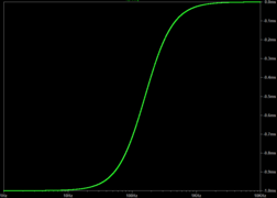
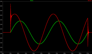
Circuit with negative group delay of = −RC = −1 ms for frequencies much lower than 1⁄RC = 1 kHz.
LTspiceAC simulation of from 1 Hz( ≅ −1 ms) to 10 kHz ( ≅ 0 ms).
Transient simulation of an input (green) wave whose output (red) is ahead by 1 ms, but with instability when the input turns on and off.
Filters will have negative group delay over frequency ranges where its phase response is positively-sloped. If a signal is band-limited within some maximum frequency B, then it is predictable to a small degree (within time periods smaller than 1⁄B). A filter whose group delay is negative over that signal's entire frequency range is able to use the signal's predictability to provide an illusion of a non-causal time advance. However, if the signal contains an unpredictable event (such as an abrupt change which makes the signal's spectrum exceed its band-limit), then the illusion breaks down.[10] Circuits with negative group delay (e.g., Figure 2) are possible, though causality is not violated.[11]
Negative group delay filters can be made in both digital and analog domains. Applications include compensating for the inherent delay of low-pass filters, to create zero phase filters, which can be used to quickly detect changes in the trends of sensor data or stock prices.[12]
Group delay in audio
Group delay has some importance in the audio field and especially in the sound reproduction field.[13][14] Many components of an audio reproduction chain, notably loudspeakers and multiway loudspeaker crossover networks, introduce group delay in the audio signal.[2][14] It is therefore important to know the threshold of audibility of group delay with respect to frequency,[15][16][17] especially if the audio chain is supposed to provide high fidelity reproduction. The best thresholds of audibility table has been provided by Blauert and Laws.[18]
Frequency (kHz)
Threshold (ms)
Periods (Cycles)
0.5
3.2
1.6
1
2
2
2
1
2
4
1.5
6
8
2
16
Flanagan, Moore and Stone conclude that at 1, 2 and 4kHz, a group delay of about 1.6ms is audible with headphones in a non-reverberant condition.[19] Other experimental results suggest that when the group delay in the frequency range from 300Hz to 1kHz is below 1.0ms, it is inaudible.[16]
The waveform of any signal can be reproduced exactly by a system that has a flat frequency response and group delay over the bandwidth of the signal. Leach[20] introduced the concept of differential time-delay distortion, defined as the difference between the phase delay and the group delay:
.
An ideal system should exhibit zero or negligible differential time-delay distortion.[20]
It is possible to use digital signal processing techniques to correct the group delay distortion that arises due to the use of crossover networks in multi-way loudspeaker systems.[21] This involves considerable computational modeling of loudspeaker systems in order to successfully apply delay equalization,[22] using the Parks-McClellan FIR equiripple filter design algorithm.[1][5][23][24]
Group delay in optics
Group delay is important in physics, and in particular in optics.
In an optical fiber, group delay is the transit time required for optical power, traveling at a given mode's group velocity, to travel a given distance. For optical fiber dispersion measurement purposes, the quantity of interest is group delay per unit length, which is the reciprocal of the group velocity of a particular mode. The measured group delay of a signal through an optical fiber exhibits a wavelength dependence due to the various dispersion mechanisms present in the fiber.
It is often desirable for the group delay to be constant across all frequencies; otherwise there is temporal smearing of the signal. Because group delay is , it therefore follows that a constant group delay can be achieved if the transfer function of the device or medium has a linear phase response (i.e., where the group delay is a constant). The degree of nonlinearity of the phase indicates the deviation of the group delay from a constant value.
The differential group delay is the difference in propagation time between the two eigenmodesX and Ypolarizations. Consider two eigenmodes that are the 0° and 90° linearpolarization states. If the state of polarization of the input signal is the linear state at 45° between the two eigenmodes, the input signal is divided equally into the two eigenmodes. The power of the transmitted signalET,total is the combination of the transmitted signals of both x and y modes.
The differential group delay Dt is defined as the difference in propagation time between the eigenmodes: Dt=|tt,x−tt,y|.
True time delay
A transmitting apparatus is said to have true time delay (TTD) if the time delay is independent of the frequency of the electrical signal.[25][26] TTD allows for a wide instantaneous signal bandwidth with virtually no signal distortion such as pulse broadening during pulsed operation.
TTD is an important characteristic of lossless and low-loss, dispersion free, transmission lines. Telegrapher's equations §Lossless transmission reveals that signals propagate through them at a speed of for a distributed inductance L and capacitance C. Hence, any signal's propagation delay through the line simply equals the length of the line divided by this speed.
to determine from , use the definition of . Given that is always real, and is always imaginary, may be redefined as where even and odd refer to the polynomials that contain only the even or odd order coefficients respectively. The in the numerator merely converts the imaginary numerator to a real value, since by itself is purely imaginary.
The above expressions contain four terms to calculate:
The equations above may be used to determine the group delay of polynomial in closed form, shown below after the equations have been reduced to a simplified form.
Polynomial ratio
A polynomial ratio of the form , such as that typically found in the definition of filter designs, may have the group delay determined by taking advantage of the phase relation, .
Simple filter example
A four pole Legendre filter transfer function used in the Legendre filter example is shown below.
The numerator group delay by inspection is zero, so only the denominator group delay need be determined.
Evaluating at = 1 rad/sec:
The group delay calculation procedure and results may be confirmed to be correct by comparing them to the results derived from the digital derivative of the phase angle, , using a small delta of +/-1.e-04 rad/sec.
Since the group delay calculated by the digital derivative using a small delta is within 7 digits of accuracy when compared to the precise analytical calculation, the group delay calculation procedure and results are confirmed to be correct.
Deviation from Linear Phase
Deviation from Linear Phase, , sometimes referred to as just, "phase deviation", is the difference between the phase response, , and the linear portion of the phase response ,[27] and is a useful measurement to determine the linearity of .
A convenient means to measure is to take the simple linear regression of sampled over a frequency range of interest, and subtract it from the actual . The of an ideal linear phase response would be expected to have a value of 0 across the frequency range of interest (such as the pass band of a filter), while the of a real-world approximately linear phase response may deviate from 0 by a small finite amount across the frequency range of interest.
Advantage over group delay
An advantage of measuring or calculating over measuring or calculating group delay, , is always converges to 0 as the phase becomes linear, whereas converges on a finite quantity that may not be known ahead of time. Given this, a linear phase optimizing function may more easily be executed with a goal than with a goal when the value for is not necessarily already known.
Linear filters process time-varying input signals to produce output signals, subject to the constraint of linearity. In most cases these linear filters are also time invariant in which case they can be analyzed exactly using LTI system theory revealing their transfer functions in the frequency domain and their impulse responses in the time domain. Real-time implementations of such linear signal processing filters in the time domain are inevitably causal, an additional constraint on their transfer functions. An analog electronic circuit consisting only of linear components will necessarily fall in this category, as will comparable mechanical systems or digital signal processing systems containing only linear elements. Since linear time-invariant filters can be completely characterized by their response to sinusoids of different frequencies, they are sometimes known as frequency filters.
In classical mechanics, a harmonic oscillator is a system that, when displaced from its equilibrium position, experiences a restoring force F proportional to the displacement x: where k is a positive constant.
In engineering, a transfer function of a system, sub-system, or component is a mathematical function that models the system's output for each possible input. It is widely used in electronic engineering tools like circuit simulators and control systems. In simple cases, this function can be represented as a two-dimensional graph of an independent scalar input versus the dependent scalar output. Transfer functions for components are used to design and analyze systems assembled from components, particularly using the block diagram technique, in electronics and control theory.
A chirp is a signal in which the frequency increases (up-chirp) or decreases (down-chirp) with time. In some sources, the term chirp is used interchangeably with sweep signal. It is commonly applied to sonar, radar, and laser systems, and to other applications, such as in spread-spectrum communications. This signal type is biologically inspired and occurs as a phenomenon due to dispersion. It is usually compensated for by using a matched filter, which can be part of the propagation channel. Depending on the specific performance measure, however, there are better techniques both for radar and communication. Since it was used in radar and space, it has been adopted also for communication standards. For automotive radar applications, it is usually called linear frequency modulated waveform (LFMW).
Angle modulation is a class of carrier modulation that is used in telecommunications transmission systems. The class comprises frequency modulation (FM) and phase modulation (PM), and is based on altering the frequency or the phase, respectively, of a carrier signal to encode the message signal. This contrasts with varying the amplitude of the carrier, practiced in amplitude modulation (AM) transmission, the earliest of the major modulation methods used widely in early radio broadcasting.
A resistor–capacitor circuit, or RC filter or RC network, is an electric circuit composed of resistors and capacitors. It may be driven by a voltage or current source and these will produce different responses. A first order RC circuit is composed of one resistor and one capacitor and is the simplest type of RC circuit.
The step response of a system in a given initial state consists of the time evolution of its outputs when its control inputs are Heaviside step functions. In electronic engineering and control theory, step response is the time behaviour of the outputs of a general system when its inputs change from zero to one in a very short time. The concept can be extended to the abstract mathematical notion of a dynamical system using an evolution parameter.
In control theory and signal processing, a linear, time-invariant system is said to be minimum-phase if the system and its inverse are causal and stable.
The Butterworth filter is a type of signal processing filter designed to have a frequency response that is as flat as possible in the passband. It is also referred to as a maximally flat magnitude filter. It was first described in 1930 by the British engineer and physicist Stephen Butterworth in his paper entitled "On the Theory of Filter Amplifiers".
In signal processing, linear phase is a property of a filter where the phase response of the filter is a linear function of frequency. The result is that all frequency components of the input signal are shifted in time by the same constant amount, which is referred to as the group delay. Consequently, there is no phase distortion due to the time delay of frequencies relative to one another.
In system analysis, among other fields of study, a linear time-invariant (LTI) system is a system that produces an output signal from any input signal subject to the constraints of linearity and time-invariance; these terms are briefly defined in the overview below. These properties apply (exactly or approximately) to many important physical systems, in which case the response y(t) of the system to an arbitrary input x(t) can be found directly using convolution: y(t) = (x ∗ h)(t) where h(t) is called the system's impulse response and ∗ represents convolution (not to be confused with multiplication). What's more, there are systematic methods for solving any such system (determining h(t)), whereas systems not meeting both properties are generally more difficult (or impossible) to solve analytically. A good example of an LTI system is any electrical circuit consisting of resistors, capacitors, inductors and linear amplifiers.
A resistor–inductor circuit, or RL filter or RL network, is an electric circuit composed of resistors and inductors driven by a voltage or current source. A first-order RL circuit is composed of one resistor and one inductor, either in series driven by a voltage source or in parallel driven by a current source. It is one of the simplest analogue infinite impulse response electronic filters.
Self-phase modulation (SPM) is a nonlinear optical effect of light–matter interaction. An ultrashort pulse of light, when travelling in a medium, will induce a varying refractive index of the medium due to the optical Kerr effect. This variation in refractive index will produce a phase shift in the pulse, leading to a change of the pulse's frequency spectrum.
Instantaneous phase and frequency are important concepts in signal processing that occur in the context of the representation and analysis of time-varying functions. The instantaneous phase (also known as local phase or simply phase) of a complex-valued function s(t), is the real-valued function:
In ultrafast optics, spectral phase interferometry for direct electric-field reconstruction (SPIDER) is an ultrashort pulse measurement technique originally developed by Chris Iaconis and Ian Walmsley.
The method of reassignment is a technique for sharpening a time-frequency representation by mapping the data to time-frequency coordinates that are nearer to the true region of support of the analyzed signal. The method has been independently introduced by several parties under various names, including method of reassignment, remapping, time-frequency reassignment, and modified moving-window method. The method of reassignment sharpens blurry time-frequency data by relocating the data according to local estimates of instantaneous frequency and group delay. This mapping to reassigned time-frequency coordinates is very precise for signals that are separable in time and frequency with respect to the analysis window.
In statistical signal processing, the goal of spectral density estimation (SDE) or simply spectral estimation is to estimate the spectral density of a signal from a sequence of time samples of the signal. Intuitively speaking, the spectral density characterizes the frequency content of the signal. One purpose of estimating the spectral density is to detect any periodicities in the data, by observing peaks at the frequencies corresponding to these periodicities.
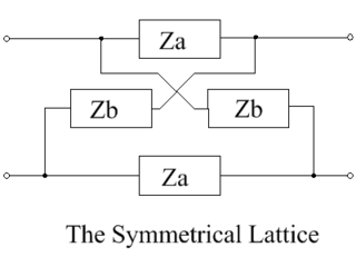
Lattice delay networks are an important subgroup of lattice networks. They are all-pass filters, so they have a flat amplitude response, but a phase response which varies linearly with frequency. All lattice circuits, regardless of their complexity, are based on the schematic shown below, which contains two series impedances, Za, and two shunt impedances, Zb. Although there is duplication of impedances in this arrangement, it offers great flexibility to the circuit designer so that, in addition to its use as delay network it can be configured to be a phase corrector, a dispersive network, an amplitude equalizer, or a low pass filter, according to the choice of components for the lattice elements.
Steered-response power (SRP) is a family of acoustic source localization algorithms that can be interpreted as a beamforming-based approach that searches for the candidate position or direction that maximizes the output of a steered delay-and-sum beamformer.
Spectral interferometry (SI) or frequency-domain interferometry is a linear technique used to measure optical pulses, with the condition that a reference pulse that was previously characterized is available. This technique provides information about the intensity and phase of the pulses. SI was first proposed by Claude Froehly and coworkers in the 1970s.
1 2 3 Rabiner, Lawrence R.; Gold, Bernard (1975). Theory and Application of Digital Signal Processing. Englewood Cliffs, New Jersey: Prentice-Hall, Inc. ISBN0-13-914101-4.
↑ Lathi, B. P. (2005). Linear Systems and Signals (Seconded.). Oxford University Press, Inc. ISBN978-0-19-515833-5.
↑ Oppenheim, Alan V.; Schafer, R. W.; Buck, J. R. (1999). Discrete-Time Signal Processing. Upper Saddle River, New Jersey: Prentice-Hall, Inc. ISBN0-13-754920-2.
1 2 Oppenheim, Alan V.; Schafer, Ronald W. (2014). Discrete-Time Signal Processing. England: Pearson Education Limited. ISBN978-1-292-02572-8.
↑ Ambardar, Ashok (1999). Analog and Digital Signal Processing (Seconded.). Cengage Learning. ISBN9780534954093.
↑ Oppenheim, Alan V.; Willsky, Alan S.; Nawab, Hamid (1997). Signals and Systems. Upper Saddle River, New Jersey: Prentice-Hall, Inc. ISBN0-13-814757-4.
↑ Bariska, Andor (2008). "Negative Group Delay"(PDF). Physical Meaning of Negative Group Delay?. Archived(PDF) from the original on 2021-10-16. Retrieved 2022-10-28.
1 2 Ashley, J. (1980). Group and phase delay requirements for loudspeaker systems. ICASSP '80. IEEE International Conference on Acoustics, Speech, and Signal Processing. Vol.5. pp.1030–1033. doi:10.1109/ICASSP.1980.1170852.
1 2 Liski, J.; Mäkivirta, A.; Välimäki, V. (2018). Audibility of loudspeaker group-delay characteristics(PDF). 144th Audio Engineering Society International Convention, Paper Number 10008. Audio Engineering Society. pp.879–888. Archived(PDF) from the original on 2022-10-09. Retrieved 2022-05-21.
↑ McClellan, J.; Parks, T.; Rabiner, L. (1973). "A computer program for designing optimum FIR linear phase digital filters". IEEE Transactions on Audio and Electroacoustics. 21 (6): 506–526. doi:10.1109/TAU.1973.1162525.
↑ Oppenheim, Alan V.; Schafer, Ronald W. (2010). Discrete-Time Signal Processing. England: Pearson Education Limited. ISBN978-0-13-198842-2.
This page is based on this Wikipedia article Text is available under the CC BY-SA 4.0 license; additional terms may apply. Images, videos and audio are available under their respective licenses.