Aharonov–Bohm effect

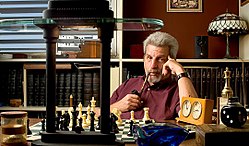
Aharonov–Bohm effect apparatus showing barrier, X; slots S₁ and S₂; electron paths e₁ and e₂; magnetic whisker, W; screen, P; interference pattern, I; magnetic flux density, B (pointing out of figure); and magnetic vector potential, A. B is essentially nil outside the whisker. In some experiments, the whisker is replaced by a solenoid. The electrons in path 1 are shifted with respect to the electrons in path 2 by the vector potential even though the flux density is nil.

Yakir Aharonov

David Bohm

The Aharonov–Bohm effect, sometimes called the Ehrenberg–Siday–Aharonov–Bohm effect, is a quantum-mechanical phenomenon in which an electrically charged particle is affected by an electromagnetic potential (${\displaystyle \varphi }$, ${\displaystyle \mathbf {A} }$), despite being confined to a region in which both the magnetic field ${\displaystyle \mathbf {B} }$ and electric field ${\displaystyle \mathbf {E} }$ are zero. ^[1] The underlying mechanism is the coupling of the electromagnetic potential with the complex phase of a charged particle's wave function, and the Aharonov–Bohm effect is accordingly illustrated by interference experiments.

The most commonly described case, sometimes called the Aharonov–Bohm solenoid effect, takes place when the wave function of a charged particle passing around a long solenoid experiences a phase shift as a result of the enclosed magnetic field, despite the magnetic field being negligible in the region through which the particle passes and the particle's wavefunction being negligible inside the solenoid. This phase shift has been observed experimentally. ^[2] There are also magnetic Aharonov–Bohm effects on bound energies and scattering cross sections, but these cases have not been experimentally tested. An electric Aharonov–Bohm phenomenon was also predicted, in which a charged particle is affected by regions with different electrical potentials but zero electric field, but this has no experimental confirmation yet. ^[2] A separate "molecular" Aharonov–Bohm effect was proposed for nuclear motion in multiply connected regions, but this has been argued to be a different kind of geometric phase as it is "neither nonlocal nor topological", depending only on local quantities along the nuclear path. ^[3]

Werner Ehrenberg (1901–1975) and Raymond E. Siday first predicted the effect in 1949. ^[4] Yakir Aharonov and David Bohm published their analysis in 1959. ^[1] After publication of the 1959 paper, Bohm was informed of Ehrenberg and Siday's work, which was acknowledged and credited in Bohm and Aharonov's subsequent 1961 paper. ^{[5] [6] [7]} The effect was confirmed experimentally, with a very large error, while Bohm was still alive. By the time the error was down to a respectable value, Bohm had died. ^[8]

Significance

In the 18th and 19th centuries, physics was dominated by Newtonian dynamics, with its emphasis on forces. Electromagnetic phenomena were elucidated by a series of experiments involving the measurement of forces between charges, currents and magnets in various configurations. Eventually, a description arose according to which charges, currents and magnets acted as local sources of propagating force fields, which then acted on other charges and currents locally through the Lorentz force law. In this framework, because one of the observed properties of the electric field was that it was irrotational, and one of the observed properties of the magnetic field was that it was divergenceless, it was possible to express an electrostatic field as the gradient of a scalar potential (e.g. Coulomb's electrostatic potential, which is mathematically analogous to the classical gravitational potential) and a stationary magnetic field as the curl of a vector potential (then a new concept – the idea of a scalar potential was already well accepted by analogy with gravitational potential). The language of potentials generalised seamlessly to the fully dynamic case but, since all physical effects were describable in terms of the fields which were the derivatives of the potentials, potentials (unlike fields) were not uniquely determined by physical effects: potentials were only defined up to an arbitrary additive constant electrostatic potential and an irrotational stationary magnetic vector potential.

The Aharonov–Bohm effect is important conceptually because it bears on three issues apparent in the recasting of (Maxwell's) classical electromagnetic theory as a gauge theory, which before the advent of quantum mechanics could be argued to be a mathematical reformulation with no physical consequences. The Aharonov–Bohm thought experiments and their experimental realization imply that the issues were not just philosophical.

The three issues are:

1. whether potentials are "physical" or just a convenient tool for calculating force fields;
2. whether action principles are fundamental;
3. the principle of locality.

Because of reasons like these, the Aharonov–Bohm effect was chosen by the New Scientist magazine as one of the "seven wonders of the quantum world". ^[9]

Potentials vs. fields

It is generally argued that the Aharonov–Bohm effect illustrates the physicality of electromagnetic potentials, Φ and A, in quantum mechanics. Classically it was possible to argue that only the electromagnetic fields are physical, while the electromagnetic potentials are purely mathematical constructs, that due to gauge freedom aren't even unique for a given electromagnetic field.

However, Vaidman has challenged this interpretation by showing that the Aharonov–Bohm effect can be explained without the use of potentials so long as one gives a full quantum mechanical treatment to the source charges that produce the electromagnetic field. ^[10] According to this view, the potential in quantum mechanics is just as physical (or non-physical) as it was classically. Aharonov, Cohen, and Rohrlich responded that the effect may be due to a local gauge potential or due to non-local gauge-invariant fields. ^[11]

Two papers published in the journal Physical Review A in 2017 have demonstrated a quantum mechanical solution for the system. Their analysis shows that the phase shift can be viewed as generated by a solenoid's vector potential acting on the electron or the electron's vector potential acting on the solenoid or the electron and solenoid currents acting on the quantized vector potential. ^{[12] [13]}

Global action vs. local forces

Similarly, the Aharonov–Bohm effect illustrates that the Lagrangian approach to dynamics, based on energies, is not just a computational aid to the Newtonian approach, based on forces. Thus the Aharonov–Bohm effect validates the view that forces are an incomplete way to formulate physics, and potential energies must be used instead. In fact Richard Feynman complained that he had been taught electromagnetism from the perspective of electromagnetic fields, and he wished later in life he had been taught to think in terms of the electromagnetic potential instead, as this would be more fundamental. ^[14] In Feynman's path-integral view of dynamics, the potential field directly changes the phase of an electron wave function, and it is these changes in phase that lead to measurable quantities.

Locality of electromagnetic effects

The Aharonov–Bohm effect shows that the local E and B fields do not contain full information about the electromagnetic field, and the electromagnetic four-potential, (Φ, A), must be used instead. By Stokes' theorem, the magnitude of the Aharonov–Bohm effect can be calculated using the electromagnetic fields alone, or using the four-potential alone. But when using just the electromagnetic fields, the effect depends on the field values in a region from which the test particle is excluded. In contrast, when using just the four-potential, the effect only depends on the potential in the region where the test particle is allowed. Therefore, one must either abandon the principle of locality, which most physicists are reluctant to do, or accept that the electromagnetic four-potential offers a more complete description of electromagnetism than the electric and magnetic fields can. On the other hand, the Aharonov–Bohm effect is crucially quantum mechanical; quantum mechanics is well known to feature non-local effects (albeit still disallowing superluminal communication), and Vaidman has argued that this is just a non-local quantum effect in a different form. ^[10]

In classical electromagnetism the two descriptions were equivalent. With the addition of quantum theory, though, the electromagnetic potentials Φ and A are seen as being more fundamental. ^[15] Despite this, all observable effects end up being expressible in terms of the electromagnetic fields, E and B. This is interesting because, while you can calculate the electromagnetic field from the four-potential, due to gauge freedom the reverse is not true.

Magnetic solenoid effect

The magnetic Aharonov–Bohm effect can be seen as a result of the requirement that quantum physics must be invariant with respect to the gauge choice for the electromagnetic potential, of which the magnetic vector potential ${\displaystyle \mathbf {A} }$ forms part.

Electromagnetic theory implies ^[16] that a particle with electric charge ${\displaystyle q}$ traveling along some path ${\displaystyle P}$ in a region with zero magnetic field ${\displaystyle \mathbf {B} }$, but non-zero ${\displaystyle \mathbf {A} }$ (by ${\displaystyle \mathbf {B} =\mathbf {0} =\nabla \times \mathbf {A} }$), acquires a phase shift ${\displaystyle \varphi }$, given in SI units by

${\displaystyle \varphi ={\frac {q}{\hbar }}\int _{P}\mathbf {A} \cdot d\mathbf {x} ,}$

Therefore, particles, with the same start and end points, but traveling along two different routes will acquire a phase difference ${\displaystyle \Delta \varphi }$ determined by the magnetic flux ${\displaystyle \Phi _{B}}$ through the area between the paths (via Stokes' theorem and ${\displaystyle \nabla \times \mathbf {A} =\mathbf {B} }$), and given by:

${\displaystyle \Delta \varphi ={\frac {q\,\Phi _{B}}{\hbar }}.}$

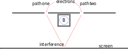
Schematic of double-slit experiment in which the Aharonov–Bohm effect can be observed: electrons pass through two slits, interfering at an observation screen, with the interference pattern shifted when a magnetic field B is changed in the whisker. The direction of the B field is outward from the figure; the inward returning flux is not shown, but is outside the electron paths. The arrow shows the direction of the A field which extends outside the boxed region even though the B field does not.

In quantum mechanics the same particle can travel between two points by a variety of paths. Therefore, this phase difference can be observed by placing a solenoid between the slits of a double-slit experiment (or equivalent). An ideal solenoid (i.e. infinitely long and with a perfectly uniform current distribution) encloses a magnetic field ${\displaystyle \mathbf {B} }$, but does not produce any magnetic field outside of its cylinder, and thus the charged particle (e.g. an electron) passing outside experiences no magnetic field ${\displaystyle \mathbf {B} }$. (This idealization simplifies the analysis but it's important to realize that the Aharonov-Bohm effect does not rely on it, provided the magnetic flux returns outside the electron paths, for example if one path goes through a toroidal solenoid and the other around it, and the solenoid is shielded so that it produces no external magnetic field.) However, there is a (curl-free) vector potential ${\displaystyle \mathbf {A} }$ outside the solenoid with an enclosed flux, and so the relative phase of particles passing through one slit or the other is altered by whether the solenoid current is turned on or off. This corresponds to an observable shift of the interference fringes on the observation plane.

The same phase effect is responsible for the quantized-flux requirement in superconducting loops. This quantization occurs because the superconducting wave function must be single valued: its phase difference ${\displaystyle \Delta \varphi }$ around a closed loop must be an integer multiple of ${\displaystyle 2\pi }$ (with the charge ${\displaystyle q=2e}$ for the electron Cooper pairs), and thus the flux must be a multiple of ${\displaystyle h/2e}$. The superconducting flux quantum was actually predicted prior to Aharonov and Bohm, by F. London in 1948 using a phenomenological model. ^[17]

The first claimed experimental confirmation was by Robert G. Chambers in 1960, ^{[18] [19]} in an electron interferometer with a magnetic field produced by a thin iron whisker, and other early work is summarized in Olariu and Popèscu (1984). ^[20] However, subsequent authors questioned the validity of several of these early results because the electrons may not have been completely shielded from the magnetic fields. ^{[21] [22] [23] [24] [25]} An early experiment in which an unambiguous Aharonov–Bohm effect was observed by completely excluding the magnetic field from the electron path (with the help of a superconducting film) was performed by Tonomura et al. in 1986. ^{[26] [27]} The effect's scope and application continues to expand. Webb et al. (1985) ^[28] demonstrated Aharonov–Bohm oscillations in ordinary, non-superconducting metallic rings; for a discussion, see Schwarzschild (1986) ^[29] and Imry & Webb (1989). ^[30] Bachtold et al. (1999) ^[31] detected the effect in carbon nanotubes; for a discussion, see Kong et al. (2004). ^[32]

Monopoles and Dirac strings

The magnetic Aharonov–Bohm effect is also closely related to Dirac's argument that the existence of a magnetic monopole can be accommodated by the existing magnetic source-free Maxwell's equations if both electric and magnetic charges are quantized.

A magnetic monopole implies a mathematical singularity in the vector potential, which can be expressed as a Dirac string of infinitesimal diameter that contains the equivalent of all of the 4πg flux from a monopole "charge" g. The Dirac string starts from, and terminates on, a magnetic monopole. Thus, assuming the absence of an infinite-range scattering effect by this arbitrary choice of singularity, the requirement of single-valued wave functions (as above) necessitates charge-quantization. That is, ${\displaystyle 2{\frac {q_{\text{e}}q_{\text{m}}}{\hbar c}}}$ must be an integer (in cgs units) for any electric charge q_e and magnetic charge q_m.

Like the electromagnetic potential A the Dirac string is not gauge invariant (it moves around with fixed endpoints under a gauge transformation) and so is also not directly measurable.

Electric effect

Just as the phase of the wave function depends upon the magnetic vector potential, it also depends upon the scalar electric potential. By constructing a situation in which the electrostatic potential varies for two paths of a particle, through regions of zero electric field, an observable Aharonov–Bohm interference phenomenon from the phase shift has been predicted; again, the absence of an electric field means that, classically, there would be no effect.

From the Schrödinger equation, the phase of an eigenfunction with energy ${\displaystyle E}$ goes as ${\displaystyle e^{-iEt/\hbar }}$. The energy, however, will depend upon the electrostatic potential ${\displaystyle V}$ for a particle with charge ${\displaystyle q}$. In particular, for a region with constant potential ${\displaystyle V}$ (zero field), the electric potential energy ${\displaystyle qV}$ is simply added to ${\displaystyle E}$, resulting in a phase shift:

${\displaystyle \Delta \varphi =-{\frac {qVt}{\hbar }},}$

where t is the time spent in the potential.

The initial theoretical proposal for this effect suggested an experiment where charges pass through conducting cylinders along two paths, which shield the particles from external electric fields in the regions where they travel, but still allow a time dependent potential to be applied by charging the cylinders. This proved difficult to realize, however. Instead, a different experiment was proposed involving a ring geometry interrupted by tunnel barriers, with a constant bias voltage V relating the potentials of the two halves of the ring. This situation results in an Aharonov–Bohm phase shift as above, and was observed experimentally in 1998, albeit in a setup where the charges do traverse the electric field generated by the bias voltage. The original time dependent electric Aharonov–Bohm effect has not yet found experimental verification. ^[33]

Gravitational effect

Main article: Gravitational Aharonov-Bohm effect

The Aharonov–Bohm phase shift due to the gravitational potential should also be possible to observe in theory, and in early 2022 ^{[34] [35] [36]} an experiment was carried out to observe it based on an experimental design from 2012. ^{[37] [38]} In the experiment, ultra-cold rubidium atoms in superposition were launched vertically inside a vacuum tube and split with a laser so that one part would go higher than the other and then recombined back. Outside of the chamber at the top sits an axially symmetric mass that changes the gravitational potential. Thus, the part that goes higher should experience a greater change which manifests as an interference pattern when the wave packets recombine resulting in a measurable phase shift. Evidence of a match between the measurements and the predictions was found by the team. Multiple other tests have been proposed. ^{[39] [40] [41] [42]}

Non-abelian effect

In 1975 Tai-Tsun Wu and Chen-Ning Yang formulated the non-Abelian Aharonov–Bohm effect, ^[43] and in 2019 this was experimentally reported in a system with light waves rather than the electron wave function. The effect was produced in two different ways. In one light went through a crystal in strong magnetic field and in another light was modulated using time-varying electrical signals. In both cases the phase shift was observed via an interference pattern which was also different depending if going forwards and backwards in time. ^{[44] [45]}

Aharonov–Bohm nano rings

Nano rings were created by accident ^[46] while intending to make quantum dots. They have interesting optical properties associated with excitons and the Aharonov–Bohm effect. ^[46] Application of these rings used as light capacitors or buffers includes photonic computing and communications technology. Analysis and measurement of geometric phases in mesoscopic rings is ongoing. ^{[47] [48] [49]} It is even suggested they could be used to make a form of slow glass. ^[50]

Several experiments, including some reported in 2012, ^[51] show Aharonov–Bohm oscillations in charge density wave (CDW) current versus magnetic flux, of dominant period h/2e through CDW rings up to 85  μm in circumference above 77 K. This behavior is similar to that of the superconducting quantum interference devices (see SQUID).

Mathematical interpretation

The Aharonov–Bohm effect can be understood from the fact that one can only measure absolute values of the wave function. While this allows for measurement of phase differences through quantum interference experiments, there is no way to specify a wavefunction with constant absolute phase. In the absence of an electromagnetic field one can come close by declaring the eigenfunction of the momentum operator with zero momentum to be the function "1" (ignoring normalization problems) and specifying wave functions relative to this eigenfunction "1". In this representation the i-momentum operator is (up to a factor ${\displaystyle \hbar /i}$) the differential operator ${\displaystyle \partial _{i}={\frac {\partial }{\partial x^{i}}}}$. However, by gauge invariance, it is equally valid to declare the zero momentum eigenfunction to be ${\displaystyle e^{-i\phi (x)}}$ at the cost of representing the i-momentum operator (up to a factor) as ${\displaystyle \nabla _{i}=\partial _{i}+i(\partial _{i}\phi )}$ i.e. with a pure gauge vector potential ${\displaystyle A=d\phi }$. There is no real asymmetry because representing the former in terms of the latter is just as messy as representing the latter in terms of the former. This means that it is physically more natural to describe wave "functions", in the language of differential geometry, as sections in a complex line bundle with a hermitian metric and a U(1)-connection ${\displaystyle \nabla }$. The curvature form of the connection, ${\displaystyle iF=\nabla \wedge \nabla }$, is, up to the factor i, the Faraday tensor of the electromagnetic field strength. The Aharonov–Bohm effect is then a manifestation of the fact that a connection with zero curvature (i.e. flat), need not be trivial since it can have monodromy along a topologically nontrivial path fully contained in the zero curvature (i.e. field-free) region. By definition this means that sections that are parallelly translated along a topologically non trivial path pick up a phase, so that covariant constant sections cannot be defined over the whole field-free region.

Given a trivialization of the line-bundle, a non-vanishing section, the U(1)-connection is given by the 1-form corresponding to the electromagnetic four-potential A as ${\displaystyle \nabla =d+iA\,}$ where d means exterior derivation on the Minkowski space. The monodromy is the holonomy of the flat connection. The holonomy of a connection, flat or non flat, around a closed loop ${\displaystyle \gamma }$ is ${\displaystyle e^{i\int _{\gamma }A}}$ (one can show this does not depend on the trivialization but only on the connection). For a flat connection one can find a gauge transformation in any simply connected field free region(acting on wave functions and connections) that gauges away the vector potential. However, if the monodromy is nontrivial, there is no such gauge transformation for the whole outside region. In fact as a consequence of Stokes' theorem, the holonomy is determined by the magnetic flux through a surface ${\displaystyle \sigma }$ bounding the loop ${\displaystyle \gamma }$, but such a surface may exist only if ${\displaystyle \sigma }$ passes through a region of non trivial field:

${\displaystyle e^{i\int _{\partial \sigma }A}=e^{i\int _{\sigma }dA}=e^{i\int _{\sigma }F}}$

The monodromy of the flat connection only depends on the topological type of the loop in the field free region (in fact on the loops homology class). The holonomy description is general, however, and works inside as well as outside the superconductor. Outside of the conducting tube containing the magnetic field, the field strength ${\displaystyle F=0}$. In other words, outside the tube the connection is flat, and the monodromy of the loop contained in the field-free region depends only on the winding number around the tube. The monodromy of the connection for a loop going round once (winding number 1) is the phase difference of a particle interfering by propagating left and right of the superconducting tube containing the magnetic field. If one wants to ignore the physics inside the superconductor and only describe the physics in the outside region, it becomes natural and mathematically convenient to describe the quantum electron by a section in a complex line bundle with an "external" flat connection ${\displaystyle \nabla }$ with monodromy

${\displaystyle \alpha =}$ magnetic flux through the tube / ${\displaystyle (\hbar /e)}$

rather than an external EM field ${\displaystyle F}$. The Schrödinger equation readily generalizes to this situation by using the Laplacian of the connection for the (free) Hamiltonian

${\displaystyle H={\frac {1}{2m}}\nabla ^{*}\nabla }$.

Equivalently, one can work in two simply connected regions with cuts that pass from the tube towards or away from the detection screen. In each of these regions the ordinary free Schrödinger equations would have to be solved, but in passing from one region to the other, in only one of the two connected components of the intersection (effectively in only one of the slits) a monodromy factor ${\displaystyle e^{i\alpha }}$ is picked up, which results in the shift in the interference pattern as one changes the flux.

Effects with similar mathematical interpretation can be found in other fields. For example, in classical statistical physics, quantization of a molecular motor motion in a stochastic environment can be interpreted as an Aharonov–Bohm effect induced by a gauge field acting in the space of control parameters. ^[52]

See also

• Geometric phase
• Hannay angle
• Wannier function
• Berry phase
• Wilson loop
• Winding number
• Aharonov–Casher effect
• Byers–Yang theorem

References

1. Aharonov, Y; Bohm, D (1959). "Significance of electromagnetic potentials in quantum theory". Physical Review . 115 (3): 485–491. Bibcode:1959PhRv..115..485A. doi: 10.1103/PhysRev.115.485 .
2. Batelaan, H. & Tonomura, A. (September 2009). "The Aharonov–Bohm effects: Variations on a Subtle Theme". Physics Today. 62 (9): 38–43. Bibcode:2009PhT....62i..38B. doi:10.1063/1.3226854.
3. Sjöqvist, E (2014). "Locality and topology in the molecular Aharonov–Bohm effect". Physical Review Letters . 89 (21): 210401. arXiv: quant-ph/0112136 . Bibcode:2002PhRvL..89u0401S. CiteSeerX   10.1.1.252.210 . doi:10.1103/PhysRevLett.89.210401. PMID   12443394. S2CID   118929792.
4. Ehrenberg, W; Siday, RE (1949). "The Refractive Index in Electron Optics and the Principles of Dynamics". Proceedings of the Physical Society B . 62 (1): 8–21. Bibcode:1949PPSB...62....8E. CiteSeerX   10.1.1.205.6343 . doi:10.1088/0370-1301/62/1/303.
5. Peat, FD (1997). Infinite Potential: The Life and Times of David Bohm . Addison-Wesley. ISBN   978-0-201-40635-1.
6. Aharonov, Y; Bohm, D (1961). "Further Considerations on Electromagnetic Potentials in the Quantum Theory". Physical Review . 123 (4): 1511–1524. Bibcode:1961PhRv..123.1511A. doi:10.1103/PhysRev.123.1511.
7. Hiley, B.J. (2013). "The Early History of the Aharonov-Bohm Effect". arXiv: 1304.4736 [physics.hist-ph].
8. Peshkin, M; Tonomura, A (1989). The Aharonov–Bohm effect. Springer-Verlag. ISBN   978-3-540-51567-8.
9. Brooks, Michael (May 5, 2010). "Seven wonders of the quantum world". New Scientist. Retrieved April 27, 2020.
10. Vaidman, L. (October 2012). "Role of potentials in the Aharonov-Bohm effect". Physical Review A. 86 (4): 040101. arXiv: 1110.6169 . Bibcode:2012PhRvA..86d0101V. doi:10.1103/PhysRevA.86.040101. S2CID   55572690.
11. Stewart, A. M. (2016). "On the paper 'Role of potentials in the Aharonov-Bohm effect'". arXiv: 1605.05470 [quant-ph].
12. P. Pearle; A. Rizzi (2017). "Quantum-mechanical inclusion of the source in the Aharonov-Bohm effects". Physical Review A. 95 (5): 052123. arXiv: 1507.00068 . Bibcode:2017PhRvA..95e2123P. doi:10.1103/PhysRevA.95.052123. S2CID   118695388.
13. P. Pearle; A. Rizzi (2017). "Quantized vector potential and alternative views of the magnetic Aharonov-Bohm phase shift". Physical Review A. 95 (5): 052124. arXiv: 1605.04324 . Bibcode:2017PhRvA..95e2124P. doi:10.1103/PhysRevA.95.052124. S2CID   119119074.
14. De Luca, Roberto; Di Mauro, Marco; Esposito, Salvatore; Naddeo, Adele (November 1, 2019). "Feynman's different approach to electromagnetism". European Journal of Physics. 40 (6): 065205. arXiv: 1902.05799 . Bibcode:2019EJPh...40f5205D. doi:10.1088/1361-6404/ab423a. S2CID   119383926.
15. Feynman, R. The Feynman Lectures on Physics. Vol. 2. pp. 15–25. knowledge of the classical electromagnetic field acting locally on a particle is not sufficient to predict its quantum-mechanical behavior. and ...is the vector potential a "real" field? ... a real field is a mathematical device for avoiding the idea of action at a distance. .... for a long time it was believed that A was not a "real" field. .... there are phenomena involving quantum mechanics which show that in fact A is a "real" field in the sense that we have defined it..... E and B are slowly disappearing from the modern expression of physical laws; they are being replaced by A [the vector potential] and ${\displaystyle \varphi }$[the scalar potential]
16. Curt Wittig. Aharonov-Bohm effect and geometric phase (PDF). pp. 200–201.
17. London, F (1948). "On the Problem of the Molecular Theory of Superconductivity". Physical Review . 74 (5): 562–573. Bibcode:1948PhRv...74..562L. doi:10.1103/PhysRev.74.562.
18. Chambers, R.G. (1960). "Shift of an Electron Interference Pattern by Enclosed Magnetic Flux". Physical Review Letters . 5 (1): 3–5. Bibcode:1960PhRvL...5....3C. doi:10.1103/PhysRevLett.5.3.
19. Popescu, S. (2010). "Dynamical quantum non-locality". Nature Physics. 6 (3): 151–153. Bibcode:2010NatPh...6..151P. doi:10.1038/nphys1619.
20. Olariu, S; Popescu, II (1985). "The quantum effects of electromagnetic fluxes". Reviews of Modern Physics . 57 (2): 339. Bibcode:1985RvMP...57..339O. doi:10.1103/RevModPhys.57.339.
21. Bocchieri, P.; Loinger, A. (1978). "Nonexistence of the Aharonov-Bohm effect". Il Nuovo Cimento A. 47 (4). Springer Science and Business Media LLC: 475–482. Bibcode:1978NCimA..47..475B. doi:10.1007/bf02896237. ISSN   0369-3546. S2CID   118437701.
22. Bocchieri, P.; Loinger, A.; Siragusa, G. (1979). "Nonexistence of the Aharonov-Bohm effect.—II". Il Nuovo Cimento A. 51 (1). Springer Science and Business Media LLC: 1–17. Bibcode:1979NCimA..51....1B. doi:10.1007/bf02822321. ISSN   0369-3546. S2CID   125804108.
23. Bocchieri, P.; Loinger, A. (1981). "Comments on the letter « on the Aharonov-Bohm effect » of Boersch et al". Lettere al Nuovo Cimento. Series 2. 30 (15). Springer Science and Business Media LLC: 449–450. doi:10.1007/bf02750508. ISSN   1827-613X. S2CID   119464057.
24. Bocchieri, P.; Loinger, A.; Siragusa, G. (1982). "Remarks on « Observation of Aharonov-Bohm effect by electron holography »". Lettere al Nuovo Cimento. Series 2. 35 (11). Springer Science and Business Media LLC: 370–372. doi:10.1007/bf02754709. ISSN   1827-613X. S2CID   123069858.
25. Roy, S. M. (January 21, 1980). "Condition for Nonexistence of Aharonov-Bohm Effect". Physical Review Letters. 44 (3). American Physical Society (APS): 111–114. Bibcode:1980PhRvL..44..111R. doi:10.1103/physrevlett.44.111. ISSN   0031-9007.
26. Tonomura, Akira; Osakabe, Nobuyuki; Matsuda, Tsuyoshi; Kawasaki, Takeshi; Endo, Junji; Yano, Shinichiro; Yamada, Hiroji (February 24, 1986). "Evidence for Aharonov-Bohm effect with magnetic field completely shielded from electron wave". Physical Review Letters. 56 (8). American Physical Society (APS): 792–795. Bibcode:1986PhRvL..56..792T. doi:10.1103/physrevlett.56.792. ISSN   0031-9007. PMID   10033287.
27. Osakabe, N; et al. (1986). "Experimental confirmation of Aharonov–Bohm effect using a toroidal magnetic field confined by a superconductor". Physical Review A . 34 (2): 815–822. Bibcode:1986PhRvA..34..815O. doi:10.1103/PhysRevA.34.815. PMID   9897338.
28. Webb, RA; Washburn, S; Umbach, CP; Laibowitz, RB (1985). "Observation of h/e Aharonov–Bohm Oscillations in Normal-Metal Rings". Physical Review Letters . 54 (25): 2696–2699. Bibcode:1985PhRvL..54.2696W. doi:10.1103/PhysRevLett.54.2696. PMID   10031414.
29. Schwarzschild, B (1986). "Currents in Normal-Metal Rings Exhibit Aharonov–Bohm Effect". Physics Today . 39 (1): 17–20. Bibcode:1986PhT....39a..17S. doi:10.1063/1.2814843.
30. Imry, Y; Webb, RA (1989). "Quantum Interference and the Aharonov–Bohm Effect". Scientific American . 260 (4): 56–62. Bibcode:1989SciAm.260d..56I. doi:10.1038/scientificamerican0489-56.
31. Schönenberger, Christian; Bachtold, Adrian; Strunk, Christoph; Salvetat, Jean-Paul; Bonard, Jean-Marc; Forró, Laszló; Nussbaumer, Thomas (1999). "Aharonov–Bohm oscillations in carbon nanotubes". Nature . 397 (6721): 673. Bibcode:1999Natur.397..673B. doi:10.1038/17755. S2CID   4429695.
32. Kong, J; Kouwenhoven, L; Dekker, C (2004). "Quantum change for nanotubes". Physics World . Retrieved August 17, 2009.
33. van Oudenaarden, A; Devoret, Michel H.; Nazarov, Yu. V.; Mooij, J. E. (1998). "Magneto-electric Aharonov–Bohm effect in metal rings". Nature . 391 (6669): 768. Bibcode:1998Natur.391..768V. doi:10.1038/35808. S2CID   4426127.
34. Overstreet, Chris; Asenbaum, Peter; Curti, Joseph; Kim, Minjeong; Kasevich, Mark A. (January 14, 2022). "Observation of a gravitational Aharonov-Bohm effect". Science. 375 (6577): 226–229. Bibcode:2022Sci...375..226O. doi:10.1126/science.abl7152. ISSN   0036-8075. PMID   35025635. S2CID   245932980.
35. "Has a new experiment just proven the quantum nature of gravity?". Big Think. January 18, 2022. Retrieved January 21, 2022.
36. "Quantum particles can feel the influence of gravitational fields they never touch". Science News. January 13, 2022. Retrieved January 21, 2022.
37. Hohensee, Michael A.; Estey, Brian; Hamilton, Paul; Zeilinger, Anton; Müller, Holger (June 7, 2012). "Force-Free Gravitational Redshift: Proposed Gravitational Aharonov-Bohm Experiment". Physical Review Letters. 108 (23): 230404. arXiv: 1109.4887 . Bibcode:2012PhRvL.108w0404H. doi:10.1103/PhysRevLett.108.230404. ISSN   0031-9007. PMID   23003927. S2CID   22378148.
38. Ehrenstein, David (June 7, 2012). "The Gravitational Aharonov-Bohm Effect". Physics. 5.
39. Dowker, J. S. (April 26, 1967). "A gravitational Aharonov-Bohm effect". Il Nuovo Cimento B. Series 10. 52 (1): 129–135. Bibcode:1967NCimB..52..129D. doi:10.1007/BF02710657. ISSN   0369-3554. S2CID   118872135.
40. Ford, L H; Vilenkin, A (September 1, 1981). "A gravitational analogue of the Aharonov-Bohm effect". Journal of Physics A: Mathematical and General. 14 (9): 2353–2357. Bibcode:1981JPhA...14.2353F. doi:10.1088/0305-4470/14/9/030. ISSN   0305-4470.
41. B Ho, Vu; J Morgan, Michael (1994). "An Experiment to Test the Gravitational Aharonov-Bohm Effect". Australian Journal of Physics. 47 (3): 245. Bibcode:1994AuJPh..47..245H. doi: 10.1071/PH940245 . ISSN   0004-9506.
42. Overstreet, Chris; Asenbaum, Peter; Kasevich, Mark A. (August 11, 2021). "Physically significant phase shifts in matter-wave interferometry". American Journal of Physics. 89 (3): 324–332. arXiv: 2008.05609 . Bibcode:2021AmJPh..89..324O. doi:10.1119/10.0002638. ISSN   0002-9505. S2CID   221113180.
43. Wu, T. T.; Yang, C. N. (1975). "Concept of non-integrable phase factors and global formulation of gauge fields". Phys. Rev. D. 12 (12): 3845–3857. Bibcode:1975PhRvD..12.3845W. doi:10.1103/PhysRevD.12.3845.
44. Yang, Yi; Peng, Chao; Zhu, Di; Buljan, Hrvoje; Joannopoulos, John D.; Zhen, Bo; Soljačić, Marin (September 6, 2019). "Synthesis and observation of non-Abelian gauge fields in real space". Science. 365 (6457): 1021–1025. arXiv: 1906.03369 . Bibcode:2019Sci...365.1021Y. doi:10.1126/science.aay3183. ISSN   0036-8075. PMID   31488687. S2CID   182953132.
45. "Non-abelian Aharonov–Bohm experiment done at long last". Physics World. October 1, 2019. Retrieved February 19, 2022.
46. Fischer, AM (2009). "Quantum doughnuts slow and freeze light at will". Innovation Reports. Archived from the original on March 31, 2009. Retrieved August 17, 2008.
47. Borunda, MF; et al. (2008). "Aharonov–Casher and spin Hall effects in two-dimensional mesoscopic ring structures with strong spin-orbit interaction". Phys. Rev. B. 78 (24): 245315. arXiv: 0809.0880 . Bibcode:2008PhRvB..78x5315B. doi:10.1103/PhysRevB.78.245315. hdl:1969.1/127350. S2CID   54723818.
48. Grbic, B; et al. (2008). "Aharonov–Bohm oscillations in p-type GaAs quantum rings". Physica E . 40 (5): 1273. arXiv: 0711.0489 . Bibcode:2008PhyE...40.1273G. doi:10.1016/j.physe.2007.08.129. S2CID   53321231.
49. Fischer, AM; et al. (2009). "Exciton Storage in a Nanoscale Aharonov–Bohm Ring with Electric Field Tuning". Physical Review Letters . 102 (9): 096405. arXiv: 0809.3863 . Bibcode:2009PhRvL.102i6405F. doi:10.1103/PhysRevLett.102.096405. PMID   19392542. S2CID   18218421.
50. "Quantum Doughnuts Slow and Freeze Light at Will: Fast Computing and 'Slow Glass'".
51. M. Tsubota; K. Inagaki; T. Matsuura & S. Tanda (2012). "Aharonov–Bohm effect in charge-density wave loops with inherent temporal current switching". EPL. 97 (5): 57011. arXiv: 0906.5206 . Bibcode:2012EL.....9757011T. doi:10.1209/0295-5075/97/57011. S2CID   119243023.
52. Chernyak, VY; Sinitsyn, NA (2009). "Robust quantization of a molecular motor motion in a stochastic environment". Journal of Chemical Physics . 131 (18): 181101. arXiv: 0906.3032 . Bibcode:2009JChPh.131r1101C. doi:10.1063/1.3263821. PMID   19916586. S2CID   14282859.

Further reading

• D. J. Thouless (1998). "§2.2 Gauge invariance and the Aharonov–Bohm effect". Topological quantum numbers in nonrelativistic physics. World Scientific. pp. 18ff. ISBN   978-981-02-3025-8.

External links

• The David Bohm Society page about the Aharonov–Bohm effect.