Definition
An inexact differential  is a differential for which the integral over some two paths with the same end points is different. Specifically, there exist integrable paths
  such that
  ,
,  and
and  In this case, we denote the integrals as
  and
and  respectively to make explicit the path dependence of the change of the quantity we are considering as
  .
.
More generally, an inexact differential is a differential form which is not an exact differential, i.e., for all functions  ,
, 
The fundamental theorem of calculus for line integrals requires path independence in order to express the values of a given vector field in terms of the partial derivatives of another function that is the multivariate analogue of the antiderivative. This is because there can be no unique representation of an antiderivative for inexact differentials since their variation is inconsistent along different paths. This stipulation of path independence is an unnecessary addendum to the fundamental theorem of calculus because in one-dimensional calculus there is only one path in between two points defined by a function.
Examples
Total distance
When you walk from a point  to a point
  along a line
  (without changing directions) your net displacement and total distance covered are both equal to the length of said line
  . If you then return to point (without changing directions) then your net displacement is zero while your total distance covered is
  . This example captures the essential idea behind the inexact differential in one dimension. Note that if we allowed ourselves to change directions, then we could take a step forward and then backward at any point in time in going from to and in-so-doing increase the overall distance covered to an arbitrarily large number while keeping the net displacement constant.
Reworking the above with differentials and taking to be along the  -axis, the net distance differential is
  , an exact differential with antiderivative . On the other hand, the total distance differential is
  , which does not have an antiderivative. The path taken is
  where there exists a time
  such that
  is strictly increasing before
  and strictly decreasing afterward. Then
  is positive before and negative afterward, yielding the integrals,
 exactly the results we expected from the verbal argument before.
First law of thermodynamics
Inexact differentials show up explicitly in the first law of thermodynamics,  where
where  is the energy,
  is the differential change in heat and
  is the differential change in work. Based on the constants of the thermodynamic system, we are able to parameterize the average energy in several different ways. E.g., in the first stage of the Carnot cycle a gas is heated by a reservoir, giving us an isothermal expansion of that gas. Some differential amount of heat
  enters the gas. During the second stage, the gas is allowed to freely expand, outputting some differential amount of work
  . The third stage is similar to the first stage, except the heat is lost by contact with a cold reservoir, while the fourth cycle is like the second except work is done onto the system by the surroundings to compress the gas. Because the overall changes in heat and work are different over different parts of the cycle, there is a nonzero net change in the heat and work, indicating that the differentials and must be inexact differentials.
Internal energy U is a state function , meaning its change can be inferred just by comparing two different states of the system (independently of its transition path), which we can therefore indicate with U1 and U2. Since we can go from state U1 to state U2 either by providing heat Q = U2 − U1 or work W = U2 − U1, such a change of state does not uniquely identify the amount of work W done to the system or heat Q transferred, but only the change in internal energy ΔU.
Heat and work
A fire requires heat, fuel, and an oxidizing agent. The energy required to overcome the activation energy barrier for combustion is transferred as heat into the system, resulting in changes to the system's internal energy. In a process, the energy input to start a fire may comprise both work and heat, such as when one rubs tinder (work) and experiences friction (heat) to start a fire. The ensuing combustion is highly exothermic, which releases heat. The overall change in internal energy does not reveal the mode of energy transfer and quantifies only the net work and heat. The difference between initial and final states of the system's internal energy does not account for the extent of the energy interactions transpired. Therefore, internal energy is a state function (i.e. exact differential), while heat and work are path functions (i.e. inexact differentials) because integration must account for the path taken.
Integrating factors
It is sometimes possible to convert an inexact differential into an exact one by means of an integrating factor. The most common example of this in thermodynamics is the definition of entropy:  In this case, δQ is an inexact differential, because its effect on the state of the system can be compensated by δW. However, when divided by the absolute temperature and when the exchange occurs at reversible conditions (therefore the rev subscript), it produces an exact differential: the entropy S is also a state function.
Example
Consider the inexact differential form,  This must be inexact by considering going to the point (1,1). If we first increase y and then increase x, then that corresponds to first integrating over y and then over x. Integrating over y first contributes
  and then integrating over x contributes
  . Thus, along the first path we get a value of 2. However, along the second path we get a value of
  . We can make an exact differential by multiplying it by x, yielding
  And so
  is an exact differential.
This page is based on this
Wikipedia article Text is available under the
CC BY-SA 4.0 license; additional terms may apply.
Images, videos and audio are available under their respective licenses.