Root system

This article is about root systems in mathematics. For plant root systems, see Root.

In mathematics, a root system is a configuration of vectors in a Euclidean space satisfying certain geometrical properties. The concept is fundamental in the theory of Lie groups and Lie algebras, especially the classification and representation theory of semisimple Lie algebras. Since Lie groups (and some analogues such as algebraic groups) and Lie algebras have become important in many parts of mathematics during the twentieth century, the apparently special nature of root systems belies the number of areas in which they are applied. Further, the classification scheme for root systems, by Dynkin diagrams, occurs in parts of mathematics with no overt connection to Lie theory (such as singularity theory). Finally, root systems are important for their own sake, as in spectral graph theory. ^[1]

Definitions and examples

The six vectors of the root system A₂

As a first example, consider the six vectors in 2-dimensional Euclidean space, R², as shown in the image at the right; call them roots. These vectors span the whole space. If you consider the line perpendicular to any root, say β, then the reflection of R² in that line sends any other root, say α, to another root. Moreover, the root to which it is sent equals α + nβ, where n is an integer (in this case, n equals 1). These six vectors satisfy the following definition, and therefore they form a root system; this one is known as A₂.

Definition

Let E be a finite-dimensional Euclidean vector space, with the standard Euclidean inner product denoted by ${\displaystyle (\cdot ,\cdot )}$. A root system${\displaystyle \Phi }$ in E is a finite set of non-zero vectors (called roots) that satisfy the following conditions: ^{[2] [3]}

1. The roots span E.
2. The only scalar multiples of a root ${\displaystyle \alpha \in \Phi }$ that belong to ${\displaystyle \Phi }$ are ${\displaystyle \alpha }$ itself and ${\displaystyle -\alpha }$.
3. For every root ${\displaystyle \alpha \in \Phi }$, the set ${\displaystyle \Phi }$ is closed under reflection through the hyperplane perpendicular to ${\displaystyle \alpha }$.
4. (Integrality) If ${\displaystyle \alpha }$ and ${\displaystyle \beta }$ are roots in ${\displaystyle \Phi }$, then the projection of ${\displaystyle \beta }$ onto the line through ${\displaystyle \alpha }$ is an integer or half-integer multiple of ${\displaystyle \alpha }$.

An equivalent way of writing conditions 3 and 4 is as follows:

3. For any two roots ${\displaystyle \alpha ,\beta \in \Phi }$, the set ${\displaystyle \Phi }$ contains the element ${\displaystyle \sigma _{\alpha }(\beta ):=\beta -2{\frac {(\alpha ,\beta )}{(\alpha ,\alpha )}}\alpha .}$
4. For any two roots ${\displaystyle \alpha ,\beta \in \Phi }$, the number ${\displaystyle \langle \beta ,\alpha \rangle$ :=2{\frac {(\alpha ,\beta )}{(\alpha ,\alpha )}}} is an integer.

Some authors only include conditions 1–3 in the definition of a root system. ^[4] In this context, a root system that also satisfies the integrality condition is known as a crystallographic root system. ^[5] Other authors omit condition 2; then they call root systems satisfying condition 2 reduced. ^[6] In this article, all root systems are assumed to be reduced and crystallographic.

In view of property 3, the integrality condition is equivalent to stating that β and its reflection σ_α(β) differ by an integer multiple of α. Note that the operator

$${\displaystyle \langle \cdot ,\cdot \rangle \colon \Phi \times \Phi \to \mathbb {Z} }$$

defined by property 4 is not an inner product. It is not necessarily symmetric and is linear only in the first argument.

Rank-2 root systems

Root system ${\displaystyle A_{1}\times A_{1}}$	Root system ${\displaystyle D_{2}}$
Root system ${\displaystyle A_{2}}$	Root system ${\displaystyle G_{2}}$
Root system ${\displaystyle B_{2}}$	Root system ${\displaystyle C_{2}}$

The rank of a root system Φ is the dimension of E. Two root systems may be combined by regarding the Euclidean spaces they span as mutually orthogonal subspaces of a common Euclidean space. A root system which does not arise from such a combination, such as the systems A₂, B₂, and G₂ pictured to the right, is said to be irreducible.

Two root systems (E₁, Φ₁) and (E₂, Φ₂) are called isomorphic if there is an invertible linear transformation E₁ → E₂ which sends Φ₁ to Φ₂ such that for each pair of roots, the number ${\displaystyle \langle x,y\rangle }$ is preserved. ^[7]

The root lattice of a root system Φ is the Z-submodule of E generated by Φ. It is a lattice in E.

Weyl group

Main article: Weyl group

The Weyl group of the ${\displaystyle A_{2}}$ root system is the symmetry group of an equilateral triangle

The group of isometries of E generated by reflections through hyperplanes associated to the roots of Φ is called the Weyl group of Φ. As it acts faithfully on the finite set Φ, the Weyl group is always finite. The reflection planes are the hyperplanes perpendicular to the roots, indicated for ${\displaystyle A_{2}}$ by dashed lines in the figure below. The Weyl group is the symmetry group of an equilateral triangle, which has six elements. In this case, the Weyl group is not the full symmetry group of the root system (e.g., a 60-degree rotation is a symmetry of the root system but not an element of the Weyl group).

Rank one example

There is only one root system of rank 1, consisting of two nonzero vectors ${\displaystyle \{\alpha ,-\alpha \}}$. This root system is called ${\displaystyle A_{1}}$.

Rank two examples

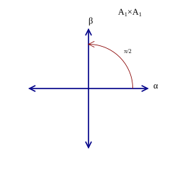
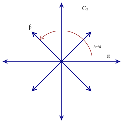
In rank 2 there are four possibilities, corresponding to ${\displaystyle \sigma _{\alpha }(\beta )=\beta +n\alpha }$, where ${\displaystyle n=0,1,2,3}$. ^[8] The figure at right shows these possibilities, but with some redundancies: ${\displaystyle A_{1}\times A_{1}}$ is isomorphic to ${\displaystyle D_{2}}$ and ${\displaystyle B_{2}}$ is isomorphic to ${\displaystyle C_{2}}$.

Note that a root system is not determined by the lattice that it generates: ${\displaystyle A_{1}\times A_{1}}$ and ${\displaystyle B_{2}}$ both generate a square lattice while ${\displaystyle A_{2}}$ and ${\displaystyle G_{2}}$ both generate a hexagonal lattice.

Whenever Φ is a root system in E, and S is a subspace of E spanned by Ψ = Φ ∩ S, then Ψ is a root system in S. Thus, the exhaustive list of four root systems of rank 2 shows the geometric possibilities for any two roots chosen from a root system of arbitrary rank. In particular, two such roots must meet at an angle of 0, 30, 45, 60, 90, 120, 135, 150, or 180 degrees.

Root systems arising from semisimple Lie algebras

See also: Semisimple Lie algebra § Cartan subalgebras and root systems, and Root system of a semi-simple Lie algebra

If ${\displaystyle {\mathfrak {g}}}$ is a complex semisimple Lie algebra and ${\displaystyle {\mathfrak {h}}}$ is a Cartan subalgebra, we can construct a root system as follows. We say that ${\displaystyle \alpha \in {\mathfrak {h}}^{*}}$ is a root of ${\displaystyle {\mathfrak {g}}}$ relative to ${\displaystyle {\mathfrak {h}}}$ if ${\displaystyle \alpha \neq 0}$ and there exists some ${\displaystyle X\neq 0\in {\mathfrak {g}}}$ such that

$${\displaystyle [H,X]=\alpha (H)X}$$

for all ${\displaystyle H\in {\mathfrak {h}}}$. One can show ^[9] that there is an inner product for which the set of roots forms a root system. The root system of ${\displaystyle {\mathfrak {g}}}$ is a fundamental tool for analyzing the structure of ${\displaystyle {\mathfrak {g}}}$ and classifying its representations. (See the section below on Root systems and Lie theory.)

History

The concept of a root system was originally introduced by Wilhelm Killing around 1889 (in German, Wurzelsystem ^[10] ). ^[11] He used them in his attempt to classify all simple Lie algebras over the field of complex numbers. Killing originally made a mistake in the classification, listing two exceptional rank 4 root systems, when in fact there is only one, now known as F₄. Cartan later corrected this mistake, by showing Killing's two root systems were isomorphic. ^[12]

Killing investigated the structure of a Lie algebra ${\displaystyle L}$, by considering what is now called a Cartan subalgebra ${\displaystyle {\mathfrak {h}}}$. Then he studied the roots of the characteristic polynomial ${\displaystyle \det(\operatorname {ad} _{L}x-t)}$, where ${\displaystyle x\in {\mathfrak {h}}}$. Here a root is considered as a function of ${\displaystyle {\mathfrak {h}}}$, or indeed as an element of the dual vector space ${\displaystyle {\mathfrak {h}}^{*}}$. This set of roots form a root system inside ${\displaystyle {\mathfrak {h}}^{*}}$, as defined above, where the inner product is the Killing form. ^[11]

Elementary consequences of the root system axioms

The integrality condition for ${\displaystyle \langle \beta ,\alpha \rangle }$ is fulfilled only for β on one of the vertical lines, while the integrality condition for ${\displaystyle \langle \alpha ,\beta \rangle }$ is fulfilled only for β on one of the red circles. Any β perpendicular to α (on the Y axis) trivially fulfills both with 0, but does not define an irreducible root system.
Modulo reflection, for a given α there are only 5 nontrivial possibilities for β, and 3 possible angles between α and β in a set of simple roots. Subscript letters correspond to the series of root systems for which the given β can serve as the first root and α as the second root (or in F₄ as the middle 2 roots).

The cosine of the angle between two roots is constrained to be one-half of the square root of a positive integer. This is because ${\displaystyle \langle \beta ,\alpha \rangle }$ and ${\displaystyle \langle \alpha ,\beta \rangle }$ are both integers, by assumption, and

$${\displaystyle {\begin{aligned}\langle \beta ,\alpha \rangle \langle \alpha ,\beta \rangle &=2{\frac {(\alpha ,\beta )}{(\alpha ,\alpha )}}\cdot 2{\frac {(\alpha ,\beta )}{(\beta ,\beta )}}\\&=4{\frac {(\alpha ,\beta )^{2}}{\vert \alpha \vert ^{2}\vert \beta \vert ^{2}}}\\&=4\cos ^{2}(\theta )=(2\cos(\theta ))^{2}\in \mathbb {Z} .\end{aligned}}}$$

Since ${\displaystyle 2\cos(\theta )\in [-2,2]}$, the only possible values for ${\displaystyle \cos(\theta )}$ are ${\displaystyle 0,\pm {\tfrac {1}{2}},\pm {\tfrac {\sqrt {2}}{2}},\pm {\tfrac {\sqrt {3}}{2}}}$ and ${\displaystyle \pm {\tfrac {\sqrt {4}}{2}}=\pm 1}$, corresponding to angles of 90°, 60° or 120°, 45° or 135°, 30° or 150°, and 0° or 180°. Condition 2 says that no scalar multiples of α other than 1 and −1 can be roots, so 0 or 180°, which would correspond to 2α or −2α, are out. The diagram at right shows that an angle of 60° or 120° corresponds to roots of equal length, while an angle of 45° or 135° corresponds to a length ratio of ${\displaystyle {\sqrt {2}}}$ and an angle of 30° or 150° corresponds to a length ratio of ${\displaystyle {\sqrt {3}}}$.

In summary, here are the only possibilities for each pair of roots. ^[13]

• Angle of 90 degrees; in that case, the length ratio is unrestricted.
• Angle of 60 or 120 degrees, with a length ratio of 1.
• Angle of 45 or 135 degrees, with a length ratio of ${\displaystyle {\sqrt {2}}}$.
• Angle of 30 or 150 degrees, with a length ratio of ${\displaystyle {\sqrt {3}}}$.

Positive roots and simple roots

The labeled roots are a set of positive roots for the ${\displaystyle G_{2}}$ root system, with ${\displaystyle \alpha _{1}}$ and ${\displaystyle \alpha _{2}}$ being the simple roots

Given a root system ${\displaystyle \Phi }$ we can always choose (in many ways) a set of positive roots. This is a subset ${\displaystyle \Phi ^{+}}$ of ${\displaystyle \Phi }$ such that

• For each root ${\displaystyle \alpha \in \Phi }$ exactly one of the roots ${\displaystyle \alpha }$, ${\displaystyle -\alpha }$ is contained in ${\displaystyle \Phi ^{+}}$.
• For any two distinct ${\displaystyle \alpha ,\beta \in \Phi ^{+}}$ such that ${\displaystyle \alpha +\beta }$ is a root, ${\displaystyle \alpha +\beta \in \Phi ^{+}}$.

If a set of positive roots ${\displaystyle \Phi ^{+}}$ is chosen, elements of ${\displaystyle -\Phi ^{+}}$ are called negative roots. A set of positive roots may be constructed by choosing a hyperplane ${\displaystyle V}$ not containing any root and setting ${\displaystyle \Phi ^{+}}$ to be all the roots lying on a fixed side of ${\displaystyle V}$. Furthermore, every set of positive roots arises in this way. ^[14]

An element of ${\displaystyle \Phi ^{+}}$ is called a simple root (also fundamental root) if it cannot be written as the sum of two elements of ${\displaystyle \Phi ^{+}}$. (The set of simple roots is also referred to as a base for ${\displaystyle \Phi }$.) The set ${\displaystyle \Delta }$ of simple roots is a basis of ${\displaystyle E}$ with the following additional special properties: ^[15]

• Every root ${\displaystyle \alpha \in \Phi }$ is a linear combination of elements of ${\displaystyle \Delta }$ with integer coefficients.
• For each ${\displaystyle \alpha \in \Phi }$, the coefficients in the previous point are either all non-negative or all non-positive.

For each root system ${\displaystyle \Phi }$ there are many different choices of the set of positive roots—or, equivalently, of the simple roots—but any two sets of positive roots differ by the action of the Weyl group. ^[16]

Dual root system, coroots, and integral elements

See also: Langlands dual group

The dual root system

If Φ is a root system in E, the coroot α^∨ of a root α is defined by

$${\displaystyle \alpha ^{\vee }={2 \over (\alpha ,\alpha )}\,\alpha .}$$

The set of coroots also forms a root system Φ^∨ in E, called the dual root system (or sometimes inverse root system). By definition, α^{∨ ∨} = α, so that Φ is the dual root system of Φ^∨. The lattice in E spanned by Φ^∨ is called the coroot lattice. Both Φ and Φ^∨ have the same Weyl group W and, for s in W,

$${\displaystyle (s\alpha )^{\vee }=s(\alpha ^{\vee }).}$$

If Δ is a set of simple roots for Φ, then Δ^∨ is a set of simple roots for Φ^∨. ^[17]

In the classification described below, the root systems of type ${\displaystyle A_{n}}$ and ${\displaystyle D_{n}}$ along with the exceptional root systems ${\displaystyle E_{6},E_{7},E_{8},F_{4},G_{2}}$ are all self-dual, meaning that the dual root system is isomorphic to the original root system. By contrast, the ${\displaystyle B_{n}}$ and ${\displaystyle C_{n}}$ root systems are dual to one another, but not isomorphic (except when ${\displaystyle n=2}$).

Integral elements

See also: Weight (representation theory) § Weights in the representation theory of semisimple Lie algebras

A vector ${\displaystyle \lambda }$ in E is called integral ^[18] if its inner product with each coroot is an integer:

$${\displaystyle 2{\frac {(\lambda ,\alpha )}{(\alpha ,\alpha )}}\in \mathbb {Z} ,\quad \alpha \in \Phi .}$$

Since the set of ${\displaystyle \alpha ^{\vee }}$ with ${\displaystyle \alpha \in \Delta }$ forms a base for the dual root system, to verify that ${\displaystyle \lambda }$ is integral, it suffices to check the above condition for ${\displaystyle \alpha \in \Delta }$.

The set of integral elements is called the weight lattice associated to the given root system. This term comes from the representation theory of semisimple Lie algebras, where the integral elements form the possible weights of finite-dimensional representations.

The definition of a root system guarantees that the roots themselves are integral elements. Thus, every integer linear combination of roots is also integral. In most cases, however, there will be integral elements that are not integer combinations of roots. That is to say, in general the weight lattice does not coincide with the root lattice.

Classification of root systems by Dynkin diagrams

See also: Dynkin diagram

Pictures of all the connected Dynkin diagrams

A root system is irreducible if it cannot be partitioned into the union of two proper subsets ${\displaystyle \Phi =\Phi _{1}\cup \Phi _{2}}$, such that ${\displaystyle (\alpha ,\beta )=0}$ for all ${\displaystyle \alpha \in \Phi _{1}}$ and ${\displaystyle \beta \in \Phi _{2}}$ .

Irreducible root systems correspond to certain graphs, the Dynkin diagrams named after Eugene Dynkin. The classification of these graphs is a simple matter of combinatorics, and induces a classification of irreducible root systems.

Constructing the Dynkin diagram

Given a root system, select a set Δ of simple roots as in the preceding section. The vertices of the associated Dynkin diagram correspond to the roots in Δ. Edges are drawn between vertices as follows, according to the angles. (Note that the angle between simple roots is always at least 90 degrees.)

• No edge if the vectors are orthogonal,
• An undirected single edge if they make an angle of 120 degrees,
• A directed double edge if they make an angle of 135 degrees, and
• A directed triple edge if they make an angle of 150 degrees.

The term "directed edge" means that double and triple edges are marked with an arrow pointing toward the shorter vector. (Thinking of the arrow as a "greater than" sign makes it clear which way the arrow is supposed to point.)

Note that by the elementary properties of roots noted above, the rules for creating the Dynkin diagram can also be described as follows. No edge if the roots are orthogonal; for nonorthogonal roots, a single, double, or triple edge according to whether the length ratio of the longer to shorter is 1, ${\displaystyle {\sqrt {2}}}$, ${\displaystyle {\sqrt {3}}}$. In the case of the ${\displaystyle G_{2}}$ root system for example, there are two simple roots at an angle of 150 degrees (with a length ratio of ${\displaystyle {\sqrt {3}}}$). Thus, the Dynkin diagram has two vertices joined by a triple edge, with an arrow pointing from the vertex associated to the longer root to the other vertex. (In this case, the arrow is a bit redundant, since the diagram is equivalent whichever way the arrow goes.)

Classifying root systems

Although a given root system has more than one possible set of simple roots, the Weyl group acts transitively on such choices. ^[19] Consequently, the Dynkin diagram is independent of the choice of simple roots; it is determined by the root system itself. Conversely, given two root systems with the same Dynkin diagram, one can match up roots, starting with the roots in the base, and show that the systems are in fact the same. ^[20]

Thus the problem of classifying root systems reduces to the problem of classifying possible Dynkin diagrams. A root systems is irreducible if and only if its Dynkin diagrams is connected. ^[21] The possible connected diagrams are as indicated in the figure. The subscripts indicate the number of vertices in the diagram (and hence the rank of the corresponding irreducible root system).

If ${\displaystyle \Phi }$ is a root system, the Dynkin diagram for the dual root system ${\displaystyle \Phi ^{\vee }}$ is obtained from the Dynkin diagram of ${\displaystyle \Phi }$ by keeping all the same vertices and edges, but reversing the directions of all arrows. Thus, we can see from their Dynkin diagrams that ${\displaystyle B_{n}}$ and ${\displaystyle C_{n}}$ are dual to each other.

Weyl chambers and the Weyl group

See also: Coxeter group § Affine Coxeter groups

The shaded region is the fundamental Weyl chamber for the base ${\displaystyle \{\alpha _{1},\alpha _{2}\}}$

If ${\displaystyle \Phi \subset E}$ is a root system, we may consider the hyperplane perpendicular to each root ${\displaystyle \alpha }$. Recall that ${\displaystyle \sigma _{\alpha }}$ denotes the reflection about the hyperplane and that the Weyl group is the group of transformations of ${\displaystyle E}$ generated by all the ${\displaystyle \sigma _{\alpha }}$'s. The complement of the set of hyperplanes is disconnected, and each connected component is called a Weyl chamber. If we have fixed a particular set Δ of simple roots, we may define the fundamental Weyl chamber associated to Δ as the set of points ${\displaystyle v\in E}$ such that ${\displaystyle (\alpha ,v)>0}$ for all ${\displaystyle \alpha \in \Delta }$.

Since the reflections ${\displaystyle \sigma _{\alpha },\,\alpha \in \Phi }$ preserve ${\displaystyle \Phi }$, they also preserve the set of hyperplanes perpendicular to the roots. Thus, each Weyl group element permutes the Weyl chambers.

The figure illustrates the case of the ${\displaystyle A_{2}}$ root system. The "hyperplanes" (in this case, one dimensional) orthogonal to the roots are indicated by dashed lines. The six 60-degree sectors are the Weyl chambers and the shaded region is the fundamental Weyl chamber associated to the indicated base.

A basic general theorem about Weyl chambers is this: ^[22]

Theorem: The Weyl group acts freely and transitively on the Weyl chambers. Thus, the order of the Weyl group is equal to the number of Weyl chambers.

In the ${\displaystyle A_{2}}$ case, for example, the Weyl group has six elements and there are six Weyl chambers.

A related result is this one: ^[23]

Theorem: Fix a Weyl chamber ${\displaystyle C}$. Then for all ${\displaystyle v\in E}$, the Weyl-orbit of ${\displaystyle v}$ contains exactly one point in the closure ${\displaystyle {\bar {C}}}$ of ${\displaystyle C}$.

Root systems and Lie theory

Irreducible root systems classify a number of related objects in Lie theory, notably the following:

• simple complex Lie algebras (see the discussion above on root systems arising from semisimple Lie algebras),
• simply connected complex Lie groups which are simple modulo centers, and
• simply connected compact Lie groups which are simple modulo centers.

In each case, the roots are non-zero weights of the adjoint representation.

We now give a brief indication of how irreducible root systems classify simple Lie algebras over ${\displaystyle \mathbb {C} }$, following the arguments in Humphreys. ^[24] A preliminary result says that a semisimple Lie algebra is simple if and only if the associated root system is irreducible. ^[25] We thus restrict attention to irreducible root systems and simple Lie algebras.

• First, we must establish that for each simple algebra ${\displaystyle {\mathfrak {g}}}$ there is only one root system. This assertion follows from the result that the Cartan subalgebra of ${\displaystyle {\mathfrak {g}}}$ is unique up to automorphism, ^[26] from which it follows that any two Cartan subalgebras give isomorphic root systems.
• Next, we need to show that for each irreducible root system, there can be at most one Lie algebra, that is, that the root system determines the Lie algebra up to isomorphism. ^[27]
• Finally, we must show that for each irreducible root system, there is an associated simple Lie algebra. This claim is obvious for the root systems of type A, B, C, and D, for which the associated Lie algebras are the classical Lie algebras. It is then possible to analyze the exceptional algebras in a case-by-case fashion. Alternatively, one can develop a systematic procedure for building a Lie algebra from a root system, using Serre's relations. ^[28]

For connections between the exceptional root systems and their Lie groups and Lie algebras see E₈, E₇, E₆, F₄, and G₂.

Properties of the irreducible root systems

Φ	|Φ|	|Φ<|	I	D	|W|
An (n ≥ 1)	n(n + 1)			n + 1	(n + 1)!
Bn (n ≥ 2)	2n2	2n	2	2	2nn!
Cn (n ≥ 3)	2n2	2n(n − 1)	2n−1	2	2nn!
Dn (n ≥ 4)	2n(n − 1)			4	2n−1n!
E6	72			3	51840
E7	126			2	2903040
E8	240			1	696729600
F4	48	24	4	1	1152
G2	12	6	3	1	12

Irreducible root systems are named according to their corresponding connected Dynkin diagrams. There are four infinite families (A_n, B_n, C_n, and D_n, called the classical root systems) and five exceptional cases (the exceptional root systems). The subscript indicates the rank of the root system.

In an irreducible root system there can be at most two values for the length (α, α)^1/2, corresponding to short and long roots. If all roots have the same length they are taken to be long by definition and the root system is said to be simply laced; this occurs in the cases A, D and E. Any two roots of the same length lie in the same orbit of the Weyl group. In the non-simply laced cases B, C, G and F, the root lattice is spanned by the short roots and the long roots span a sublattice, invariant under the Weyl group, equal to r²/2 times the coroot lattice, where r is the length of a long root.

In the adjacent table, |Φ^<| denotes the number of short roots, I denotes the index in the root lattice of the sublattice generated by long roots, D denotes the determinant of the Cartan matrix, and |W| denotes the order of the Weyl group.

Explicit construction of the irreducible root systems

A_n

Model of the ${\displaystyle A_{3}}$ root system in the Zometool system

Simple roots in A₃

	e1	e2	e3	e4
α1	1	−1	0	0
α2	0	1	−1	0
α3	0	0	1	−1

Let E be the subspace of Rⁿ⁺¹ for which the coordinates sum to 0, and let Φ be the set of vectors in E of length √2 and which are integer vectors, i.e. have integer coordinates in Rⁿ⁺¹. Such a vector must have all but two coordinates equal to 0, one coordinate equal to 1, and one equal to −1, so there are n² + n roots in all. One choice of simple roots expressed in the standard basis is α_i = e_i − e_i+1 for 1 ≤ i ≤ n.

The reflection σ_i through the hyperplane perpendicular to α_i is the same as permutation of the adjacent ith and (i + 1)th coordinates. Such transpositions generate the full permutation group. For adjacent simple roots, σ_i(α_i+1) = α_i+1 + α_i = σ_i+1(α_i) = α_i + α_i+1, that is, reflection is equivalent to adding a multiple of 1; but reflection of a simple root perpendicular to a nonadjacent simple root leaves it unchanged, differing by a multiple of 0.

The A_n root lattice – that is, the lattice generated by the A_n roots – is most easily described as the set of integer vectors in Rⁿ⁺¹ whose components sum to zero.

The A₂ root lattice is the vertex arrangement of the triangular tiling.

The A₃ root lattice is known to crystallographers as the face-centered cubic (or cubic close packed) lattice. ^[29] It is the vertex arrangement of the tetrahedral-octahedral honeycomb.

The A₃ root system (as well as the other rank-three root systems) may be modeled in the Zometool Construction set. ^[30]

In general, the A_n root lattice is the vertex arrangement of the n-dimensional simplectic honeycomb.

B_n

Simple roots in B₄

	e1	e2	e3	e4
α1	1	−1	0	0
α2	0	1	−1	0
α3	0	0	1	−1
α4	0	0	0	1

Let E = Rⁿ, and let Φ consist of all integer vectors in E of length 1 or √2. The total number of roots is 2n². One choice of simple roots is α_i = e_i – e_i+1 for 1 ≤ i ≤ n – 1 (the above choice of simple roots for A_n−1), and the shorter root α_n = e_n.

The reflection σ_n through the hyperplane perpendicular to the short root α_n is of course simply negation of the nth coordinate. For the long simple root α_n−1, σ_n−1(α_n) = α_n + α_n−1, but for reflection perpendicular to the short root, σ_n(α_n−1) = α_n−1 + 2α_n, a difference by a multiple of 2 instead of 1.

The B_n root lattice—that is, the lattice generated by the B_n roots—consists of all integer vectors.

B₁ is isomorphic to A₁ via scaling by √2, and is therefore not a distinct root system.

C_n

Root system B₃, C₃, and A₃ = D₃ as points within a cube and octahedron

Simple roots in C₄

	e1	e2	e3	e4
α1	1	−1	0	0
α2	0	1	−1	0
α3	0	0	1	−1
α4	0	0	0	2

Let E = Rⁿ, and let Φ consist of all integer vectors in E of length √2 together with all vectors of the form 2λ, where λ is an integer vector of length 1. The total number of roots is 2n². One choice of simple roots is: α_i = e_i − e_i+1, for 1 ≤ i ≤ n − 1 (the above choice of simple roots for A_n−1), and the longer root α_n = 2e_n. The reflection σ_n(α_n−1) = α_n−1 + α_n, but σ_n−1(α_n) = α_n + 2α_n−1.

The C_n root lattice—that is, the lattice generated by the C_n roots—consists of all integer vectors whose components sum to an even integer.

C₂ is isomorphic to B₂ via scaling by √2 and a 45 degree rotation, and is therefore not a distinct root system.

D_n

Simple roots in D₄

	e1	e2	e3	e4
α1	1	−1	0	0
α2	0	1	−1	0
α3	0	0	1	−1
α4	0	0	1	1

Let E = Rⁿ, and let Φ consist of all integer vectors in E of length √2. The total number of roots is 2n(n − 1). One choice of simple roots is α_i = e_i − e_i+1 for 1 ≤ i ≤ n − 1 (the above choice of simple roots for A_n−1) together with α_n = e_n−1 + e_n.

Reflection through the hyperplane perpendicular to α_n is the same as transposing and negating the adjacent n-th and (n − 1)-th coordinates. Any simple root and its reflection perpendicular to another simple root differ by a multiple of 0 or 1 of the second root, not by any greater multiple.

The D_n root lattice – that is, the lattice generated by the D_n roots – consists of all integer vectors whose components sum to an even integer. This is the same as the C_n root lattice.

The D_n roots are expressed as the vertices of a rectified n-orthoplex, Coxeter–Dynkin diagram: .... The 2n(n − 1) vertices exist in the middle of the edges of the n-orthoplex.

D₃ coincides with A₃, and is therefore not a distinct root system. The twelve D₃ root vectors are expressed as the vertices of , a lower symmetry construction of the cuboctahedron.

D₄ has additional symmetry called triality. The twenty-four D₄ root vectors are expressed as the vertices of , a lower symmetry construction of the 24-cell.

E₆, E₇, E₈

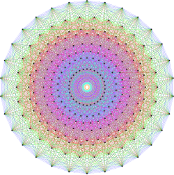
72 vertices of 122 represent the root vectors of E6 (Green nodes are doubled in this E6 Coxeter plane projection)	126 vertices of 231 represent the root vectors of E7	240 vertices of 421 represent the root vectors of E8

• The E₈ root system is any set of vectors in R⁸ that is congruent to the following set:
  $${\displaystyle D_{8}\cup \left\{{\frac {1}{2}}\left(\sum _{i=1}^{8}\varepsilon _{i}\mathbf {e} _{i}\right):\varepsilon _{i}=\pm 1,\,\varepsilon _{1}\cdots \varepsilon _{8}=+1\right\}.}$$

The root system has 240 roots. The set just listed is the set of vectors of length √2 in the E8 root lattice, also known simply as the E8 lattice or Γ₈. This is the set of points in R⁸ such that:

1. all the coordinates are integers or all the coordinates are half-integers (a mixture of integers and half-integers is not allowed), and
2. the sum of the eight coordinates is an even integer.

Thus,

$${\displaystyle E_{8}=\left\{\alpha \in \mathbb {Z} ^{8}\cup \left(\mathbb {Z} +{\tfrac {1}{2}}\right)^{8}:|\alpha |^{2}=\sum \alpha _{i}^{2}=2,\,\sum \alpha _{i}\in 2\mathbb {Z} .\right\}}$$

• The root system E₇ is the set of vectors in E₈ that are perpendicular to a fixed root in E₈. The root system E₇ has 126 roots.
• The root system E₆ is not the set of vectors in E₇ that are perpendicular to a fixed root in E₇, indeed, one obtains D₆ that way. However, E₆ is the subsystem of E₈ perpendicular to two suitably chosen roots of E₈. The root system E₆ has 72 roots.

Simple roots in E₈: even coordinates

1	−1	0	0	0	0	0	0
0	1	−1	0	0	0	0	0
0	0	1	−1	0	0	0	0
0	0	0	1	−1	0	0	0
0	0	0	0	1	−1	0	0
0	0	0	0	0	1	−1	0
0	0	0	0	0	1	1	0
−1/2	−1/2	−1/2	−1/2	−1/2	−1/2	−1/2	−1/2

An alternative description of the E₈ lattice which is sometimes convenient is as the set Γ'₈ of all points in R⁸ such that

• all the coordinates are integers and the sum of the coordinates is even, or
• all the coordinates are half-integers and the sum of the coordinates is odd.

The lattices Γ₈ and Γ'₈ are isomorphic; one may pass from one to the other by changing the signs of any odd number of coordinates. The lattice Γ₈ is sometimes called the even coordinate system for E₈ while the lattice Γ'₈ is called the odd coordinate system.

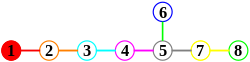
One choice of simple roots for E₈ in the even coordinate system with rows ordered by node order in the alternate (non-canonical) Dynkin diagrams (above) is:

α_i = e_i − e_i+1, for 1 ≤ i ≤ 6, and

α₇ = e₇ + e₆

(the above choice of simple roots for D₇) along with

$${\displaystyle {\boldsymbol {\alpha }}_{8}={\boldsymbol {\beta }}_{0}=-{\frac {1}{2}}\sum _{i=1}^{8}\mathbf {e} _{i}=(-1/2,-1/2,-1/2,-1/2,-1/2,-1/2,-1/2,-1/2).}$$

Simple roots in E₈: odd coordinates

1	−1	0	0	0	0	0	0
0	1	−1	0	0	0	0	0
0	0	1	−1	0	0	0	0
0	0	0	1	−1	0	0	0
0	0	0	0	1	−1	0	0
0	0	0	0	0	1	−1	0
0	0	0	0	0	0	1	−1
−1/2	−1/2	−1/2	−1/2	−1/2	1/2	1/2	1/2

One choice of simple roots for E₈ in the odd coordinate system with rows ordered by node order in alternate (non-canonical) Dynkin diagrams (above) is

α_i = e_i − e_i+1, for 1 ≤ i ≤ 7

(the above choice of simple roots for A₇) along with

α₈ = β₅, where

${\textstyle {\boldsymbol {\beta }}_{j}={\frac {1}{2}}\left(-\sum _{i=1}^{j}e_{i}+\sum _{i=j+1}^{8}e_{i}\right).}$

(Using β₃ would give an isomorphic result. Using β_1,7 or β_2,6 would simply give A₈ or D₈. As for β₄, its coordinates sum to 0, and the same is true for α_1...7, so they span only the 7-dimensional subspace for which the coordinates sum to 0; in fact −2β₄ has coordinates (1,2,3,4,3,2,1) in the basis (α_i).)

Since perpendicularity to α₁ means that the first two coordinates are equal, E₇ is then the subset of E₈ where the first two coordinates are equal, and similarly E₆ is the subset of E₈ where the first three coordinates are equal. This facilitates explicit definitions of E₇ and E₆ as

E₇ = {α ∈ Z⁷ ∪ (Z+1/2)⁷ : Σα_i² + α₁² = 2, Σα_i + α₁ ∈ 2Z},

E₆ = {α ∈ Z⁶ ∪ (Z+1/2)⁶ : Σα_i² + 2α₁² = 2, Σα_i + 2α₁ ∈ 2Z}

Note that deleting α₁ and then α₂ gives sets of simple roots for E₇ and E₆. However, these sets of simple roots are in different E₇ and E₆ subspaces of E₈ than the ones written above, since they are not orthogonal to α₁ or α₂.

F₄

Simple roots in F₄

	e1	e2	e3	e4
α1	1	−1	0	0
α2	0	1	−1	0
α3	0	0	1	0
α4	−1/2	−1/2	−1/2	−1/2

48-root vectors of F4, defined by vertices of the 24-cell and its dual, viewed in the Coxeter plane

For F₄, let E = R⁴, and let Φ denote the set of vectors α of length 1 or √2 such that the coordinates of 2α are all integers and are either all even or all odd. There are 48 roots in this system. One choice of simple roots is: the choice of simple roots given above for B₃, plus ${\textstyle {\boldsymbol {\alpha }}_{4}=-{\frac {1}{2}}\sum _{i=1}^{4}e_{i}}$.

The F₄ root lattice—that is, the lattice generated by the F₄ root system—is the set of points in R⁴ such that either all the coordinates are integers or all the coordinates are half-integers (a mixture of integers and half-integers is not allowed). This lattice is isomorphic to the lattice of Hurwitz quaternions.

G₂

Simple roots in G₂

	e1	e2	e3
α1	1	−1	0
β	−1	2	−1

The root system G₂ has 12 roots, which form the vertices of a hexagram. See the picture above.

One choice of simple roots is (α₁, β = α₂ − α₁) where α_i = e_i − e_i+1 for i = 1, 2 is the above choice of simple roots for A₂.

The G₂ root lattice—that is, the lattice generated by the G₂ roots—is the same as the A₂ root lattice.

The root poset

Hasse diagram of E6 root poset with edge labels identifying added simple root position

The set of positive roots is naturally ordered by saying that ${\displaystyle \alpha \leq \beta }$ if and only if ${\displaystyle \beta -\alpha }$ is a nonnegative linear combination of simple roots. This poset is graded by ${\textstyle \deg \left(\sum _{\alpha \in \Delta }\lambda _{\alpha }\alpha \right)=\sum _{\alpha \in \Delta }\lambda _{\alpha }}$, and has many remarkable combinatorial properties, one of them being that one can determine the degrees of the fundamental invariants of the corresponding Weyl group from this poset. ^[31] The Hasse graph is a visualization of the ordering of the root poset.

See also

• ADE classification
• Affine root system
• Coxeter–Dynkin diagram
• Coxeter group
• Coxeter matrix
• Dynkin diagram
• root datum
• Semisimple Lie algebra
• Weights in the representation theory of semisimple Lie algebras
• Root system of a semi-simple Lie algebra
• Weyl group

Notes

1. Cvetković, Dragoš (2002). "Graphs with least eigenvalue −2; a historical survey and recent developments in maximal exceptional graphs". Linear Algebra and Its Applications. 356 (1–3): 189–210. doi: 10.1016/S0024-3795(02)00377-4 .
2. Bourbaki, Ch.VI, Section 1
3. Humphreys 1972 , p. 42
4. Humphreys 1992 , p. 6
5. Humphreys 1992 , p. 39
6. Humphreys 1992 , p. 41
7. Humphreys 1972 , p. 43
8. Hall 2015 Proposition 8.8
9. Hall 2015 , Section 7.5
10. Killing 1889
11. Bourbaki 1998 , p. 270
12. Coleman 1989 , p. 34
13. Hall 2015 Proposition 8.6
14. Hall 2015 , Theorems 8.16 and 8.17
15. Hall 2015 , Theorem 8.16
16. Hall 2015 , Proposition 8.28
17. Hall 2015 , Proposition 8.18
18. Hall 2015 , Section 8.7
19. This follows from Hall 2015 , Proposition 8.23
20. Hall 2015 , Proposition 8.32
21. Hall 2015 , Proposition 8.23
22. Hall 2015 , Propositions 8.23 and 8.27
23. Hall 2015 , Proposition 8.29
24. See various parts of Chapters III, IV, and V of Humphreys 1972, culminating in Section 19 in Chapter V
25. Hall 2015, Theorem 7.35
26. Humphreys 1972 , Section 16
27. Humphreys 1972 , Part (b) of Theorem 18.4
28. Humphreys 1972 Section 18.3 and Theorem 18.4
29. Conway, John; Sloane, Neil J.A. (1998). "Section 6.3". Sphere Packings, Lattices and Groups. Springer. ISBN   978-0-387-98585-5.
30. Hall 2015 Section 8.9
31. Humphreys 1992 , Theorem 3.20

References

• Adams, J.F. (1983), Lectures on Lie groups, University of Chicago Press, ISBN   0-226-00530-5
• Bourbaki, Nicolas (2002), Lie groups and Lie algebras, Chapters 4–6 (translated from the 1968 French original by Andrew Pressley), Elements of Mathematics, Springer-Verlag, ISBN   3-540-42650-7 . The classic reference for root systems.
• Bourbaki, Nicolas (1998). Elements of the History of Mathematics . Springer. ISBN   3540647678.
• Coleman, A.J. (Summer 1989), "The greatest mathematical paper of all time", The Mathematical Intelligencer, 11 (3): 29–38, doi:10.1007/bf03025189, S2CID   35487310
• Hall, Brian C. (2015), Lie groups, Lie algebras, and representations: An elementary introduction, Graduate Texts in Mathematics, vol. 222 (2nd ed.), Springer, ISBN   978-3319134666
• Humphreys, James (1972). Introduction to Lie algebras and Representation Theory . Springer. ISBN   0387900535.
• Humphreys, James (1992). Reflection Groups and Coxeter Groups. Cambridge University Press. ISBN   0521436133.
• Killing, Wilhelm (June 1888). "Die Zusammensetzung der stetigen endlichen Transformationsgruppen". Mathematische Annalen . 31 (2): 252–290. doi:10.1007/BF01211904. S2CID   120501356. Archived from the original on 2016-03-05.
  • — (March 1888). "Part 2". Math. Ann. 33 (1): 1–48. doi:10.1007/BF01444109. S2CID   124198118.
  • — (March 1889). "Part 3". Math. Ann. 34 (1): 57–122. doi:10.1007/BF01446792. S2CID   179177899. Archived from the original on 2015-02-21.
  • — (June 1890). "Part 4". Math. Ann. 36 (2): 161–189. doi:10.1007/BF01207837. S2CID   179178061.
• Kac, Victor G. (1990). Infinite-Dimensional Lie Algebras (3rd ed.). Cambridge University Press. ISBN   978-0-521-46693-6.
• Springer, T.A. (1998). Linear Algebraic Groups (2nd ed.). Birkhäuser. ISBN   0817640215.

Further reading

• Dynkin, E.B. (1947). "The structure of semi-simple algebras". Uspekhi Mat. Nauk. 2 (in Russian). 4 (20): 59–127. MR   0027752.