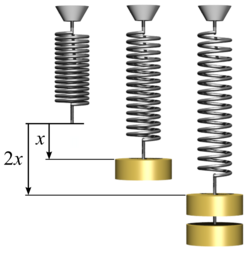
Hooke's law

Hooke's law: the force is proportional to the extension

Bourdon tubes are based on Hooke's law. The force created by gas pressure inside the coiled metal tube above unwinds it by an amount proportional to the pressure.

The balance wheel at the core of many mechanical clocks and watches depends on Hooke's law. Since the torque generated by the coiled spring is proportional to the angle turned by the wheel, its oscillations have a nearly constant period.

In physics, Hooke's law is an empirical law which states that the force (F) needed to extend or compress a spring by some distance (x) scales linearly with respect to that distance—that is, F_s = kx, where k is a constant factor characteristic of the spring (i.e., its stiffness), and x is small compared to the total possible deformation of the spring. The law is named after 17th-century British physicist Robert Hooke. He first stated the law in 1676 as a Latin anagram. ^{[1] [2]} He published the solution of his anagram in 1678 ^[3] as: ut tensio, sic vis ("as the extension, so the force" or "the extension is proportional to the force"). Hooke states in the 1678 work that he was aware of the law since 1660.

Hooke's equation holds (to some extent) in many other situations where an elastic body is deformed, such as wind blowing on a tall building, and a musician plucking a string of a guitar. An elastic body or material for which this equation can be assumed is said to be linear-elastic or Hookean.

Hooke's law is only a first-order linear approximation to the real response of springs and other elastic bodies to applied forces. It must eventually fail once the forces exceed some limit, since no material can be compressed beyond a certain minimum size, or stretched beyond a maximum size, without some permanent deformation or change of state. Many materials will noticeably deviate from Hooke's law well before those elastic limits are reached.

On the other hand, Hooke's law is an accurate approximation for most solid bodies, as long as the forces and deformations are small enough. For this reason, Hooke's law is extensively used in all branches of science and engineering, and is the foundation of many disciplines such as seismology, molecular mechanics and acoustics. It is also the fundamental principle behind the spring scale, the manometer, the galvanometer, and the balance wheel of the mechanical clock.

The modern theory of elasticity generalizes Hooke's law to say that the strain (deformation) of an elastic object or material is proportional to the stress applied to it. However, since general stresses and strains may have multiple independent components, the "proportionality factor" may no longer be just a single real number, but rather a linear map (a tensor) that can be represented by a matrix of real numbers.

In this general form, Hooke's law makes it possible to deduce the relation between strain and stress for complex objects in terms of intrinsic properties of the materials they are made of. For example, one can deduce that a homogeneous rod with uniform cross section will behave like a simple spring when stretched, with a stiffness k directly proportional to its cross-section area and inversely proportional to its length.

Formal definition

Linear springs

Elongation and compression of a spring

Consider a simple helical spring that has one end attached to some fixed object, while the free end is being pulled by a force whose magnitude is F_s. Suppose that the spring has reached a state of equilibrium, where its length is not changing anymore. Let x be the amount by which the free end of the spring was displaced from its "relaxed" position (when it is not being stretched). Hooke's law states that

$${\displaystyle F_{s}=kx}$$

or, equivalently,

$${\displaystyle x={\frac {F_{s}}{k}}}$$

where k is a positive real number, characteristic of the spring. A spring with spaces between the coils can be compressed, and the same formula holds for compression, with F_s and x both negative in that case. ^[4]

Graphical derivation

According to this formula, the graph of the applied force F_s as a function of the displacement x will be a straight line passing through the origin, whose slope is k.

Hooke's law for a spring is also stated under the convention that F_s is the restoring force exerted by the spring on whatever is pulling its free end. In that case, the equation becomes

$${\displaystyle F_{s}=-kx}$$

since the direction of the restoring force is opposite to that of the displacement.

Torsional springs

The torsional analog of Hooke's law applies to torsional springs. It states that the torque (τ) required to rotate an object is directly proportional to the angular displacement (θ) from the equilibrium position. It describes the relationship between the torque applied to an object and the resulting angular deformation due to torsion. Mathematically, it can be expressed as:

${\displaystyle \tau =-k\theta }$

Where:

• τ is the torque measured in Newton-meters or N·m.
• k is the torsional constant (measured in N·m/radian), which characterizes the stiffness of the torsional spring or the resistance to angular displacement.
• θ is the angular displacement (measured in radians) from the equilibrium position.

Just as in the linear case, this law shows that the torque is proportional to the angular displacement, and the negative sign indicates that the torque acts in a direction opposite to the angular displacement, providing a restoring force to bring the system back to equilibrium.

General "scalar" springs

Hooke's spring law usually applies to any elastic object, of arbitrary complexity, as long as both the deformation and the stress can be expressed by a single number that can be both positive and negative.

For example, when a block of rubber attached to two parallel plates is deformed by shearing, rather than stretching or compression, the shearing force F_s and the sideways displacement of the plates x obey Hooke's law (for small enough deformations).

Hooke's law also applies when a straight steel bar or concrete beam (like the one used in buildings), supported at both ends, is bent by a weight F placed at some intermediate point. The displacement x in this case is the deviation of the beam, measured in the transversal direction, relative to its unloaded shape.

Vector formulation

In the case of a helical spring that is stretched or compressed along its axis, the applied (or restoring) force and the resulting elongation or compression have the same direction (which is the direction of said axis). Therefore, if F_s and x are defined as vectors, Hooke's equation still holds and says that the force vector is the elongation vector multiplied by a fixed scalar.

General tensor form

Some elastic bodies will deform in one direction when subjected to a force with a different direction. One example is a horizontal wood beam with non-square rectangular cross section that is bent by a transverse load that is neither vertical nor horizontal. In such cases, the magnitude of the displacement x will be proportional to the magnitude of the force F_s, as long as the direction of the latter remains the same (and its value is not too large); so the scalar version of Hooke's law F_s = −kx will hold. However, the force and displacement vectors will not be scalar multiples of each other, since they have different directions. Moreover, the ratio k between their magnitudes will depend on the direction of the vector F_s.

Yet, in such cases there is often a fixed linear relation between the force and deformation vectors, as long as they are small enough. Namely, there is a function κ from vectors to vectors, such that F = κ(X), and κ(αX₁ + βX₂) = ακ(X₁) + βκ(X₂) for any real numbers α, β and any displacement vectors X₁, X₂. Such a function is called a (second-order) tensor.

With respect to an arbitrary Cartesian coordinate system, the force and displacement vectors can be represented by 3 × 1 matrices of real numbers. Then the tensor κ connecting them can be represented by a 3 × 3 matrix κ of real coefficients, that, when multiplied by the displacement vector, gives the force vector:

$${\displaystyle \mathbf {F} \,=\,{\begin{bmatrix}F_{1}\\F_{2}\\F_{3}\end{bmatrix}}\,=\,{\begin{bmatrix}\kappa _{11}&\kappa _{12}&\kappa _{13}\\\kappa _{21}&\kappa _{22}&\kappa _{23}\\\kappa _{31}&\kappa _{32}&\kappa _{33}\end{bmatrix}}{\begin{bmatrix}X_{1}\\X_{2}\\X_{3}\end{bmatrix}}\,=\,{\boldsymbol {\kappa }}\mathbf {X} }$$

That is,

$${\displaystyle F_{i}=\kappa _{i1}X_{1}+\kappa _{i2}X_{2}+\kappa _{i3}X_{3}}$$

for i = 1, 2, 3. Therefore, Hooke's law F = κX can be said to hold also when X and F are vectors with variable directions, except that the stiffness of the object is a tensor κ, rather than a single real number k.

Hooke's law for continuous media

Main article: linear elasticity

(a) Schematic of a polymer nanospring. The coil radius, R, pitch, P, length of the spring, L, and the number of turns, N, are 2.5 μm, 2.0 μm, 13 μm, and 4, respectively. Electron micrographs of the nanospring, before loading (b-e), stretched (f), compressed (g), bent (h), and recovered (i). All scale bars are 2 μm. The spring followed a linear response against applied force, demonstrating the validity of Hooke's law at the nanoscale.

The stresses and strains of the material inside a continuous elastic material (such as a block of rubber, the wall of a boiler, or a steel bar) are connected by a linear relationship that is mathematically similar to Hooke's spring law, and is often referred to by that name.

However, the strain state in a solid medium around some point cannot be described by a single vector. The same parcel of material, no matter how small, can be compressed, stretched, and sheared at the same time, along different directions. Likewise, the stresses in that parcel can be at once pushing, pulling, and shearing.

In order to capture this complexity, the relevant state of the medium around a point must be represented by two-second-order tensors, the strain tensor ε (in lieu of the displacement X) and the stress tensor σ (replacing the restoring force F). The analogue of Hooke's spring law for continuous media is then

$${\displaystyle {\boldsymbol {\sigma }}=\mathbf {c} {\boldsymbol {\varepsilon }},}$$

where c is a fourth-order tensor (that is, a linear map between second-order tensors) usually called the stiffness tensor or elasticity tensor. One may also write it as

$${\displaystyle {\boldsymbol {\varepsilon }}=\mathbf {s} {\boldsymbol {\sigma }},}$$

where the tensor s, called the compliance tensor, represents the inverse of said linear map.

In a Cartesian coordinate system, the stress and strain tensors can be represented by 3 × 3 matrices

$${\displaystyle {\boldsymbol {\varepsilon }}\,=\,{\begin{bmatrix}\varepsilon _{11}&\varepsilon _{12}&\varepsilon _{13}\\\varepsilon _{21}&\varepsilon _{22}&\varepsilon _{23}\\\varepsilon _{31}&\varepsilon _{32}&\varepsilon _{33}\end{bmatrix}}\,;\qquad {\boldsymbol {\sigma }}\,=\,{\begin{bmatrix}\sigma _{11}&\sigma _{12}&\sigma _{13}\\\sigma _{21}&\sigma _{22}&\sigma _{23}\\\sigma _{31}&\sigma _{32}&\sigma _{33}\end{bmatrix}}}$$

Being a linear mapping between the nine numbers σ_ij and the nine numbers ε_kl, the stiffness tensor c is represented by a matrix of 3 × 3 × 3 × 3 = 81 real numbers c_ijkl. Hooke's law then says that

$${\displaystyle \sigma _{ij}=\sum _{k=1}^{3}\sum _{l=1}^{3}c_{ijkl}\varepsilon _{kl}}$$

where i,j = 1,2,3.

All three tensors generally vary from point to point inside the medium, and may vary with time as well. The strain tensor ε merely specifies the displacement of the medium particles in the neighborhood of the point, while the stress tensor σ specifies the forces that neighboring parcels of the medium are exerting on each other. Therefore, they are independent of the composition and physical state of the material. The stiffness tensor c, on the other hand, is a property of the material, and often depends on physical state variables such as temperature, pressure, and microstructure.

Due to the inherent symmetries of σ, ε, and c, only 21 elastic coefficients of the latter are independent. ^[6] This number can be further reduced by the symmetry of the material: 9 for an orthorhombic crystal, 5 for an hexagonal structure, and 3 for a cubic symmetry. ^[7] For isotropic media (which have the same physical properties in any direction), c can be reduced to only two independent numbers, the bulk modulus K and the shear modulus G, that quantify the material's resistance to changes in volume and to shearing deformations, respectively.

Analogous laws

Since Hooke's law is a simple proportionality between two quantities, its formulas and consequences are mathematically similar to those of many other physical laws, such as those describing the motion of fluids, or the polarization of a dielectric by an electric field.

In particular, the tensor equation σ = cε relating elastic stresses to strains is entirely similar to the equation τ = με̇ relating the viscous stress tensor τ and the strain rate tensor ε̇ in flows of viscous fluids; although the former pertains to static stresses (related to amount of deformation) while the latter pertains to dynamical stresses (related to the rate of deformation).

Units of measurement

In SI units, displacements are measured in meters (m), and forces in newtons (N or kg·m/s²). Therefore, the spring constant k, and each element of the tensor κ, is measured in newtons per meter (N/m), or kilograms per second squared (kg/s²).

For continuous media, each element of the stress tensor σ is a force divided by an area; it is therefore measured in units of pressure, namely pascals (Pa, or N/m², or kg/(m·s²). The elements of the strain tensor ε are dimensionless (displacements divided by distances). Therefore, the entries of c_ijkl are also expressed in units of pressure.

General application to elastic materials

Stress–strain curve for low-carbon steel, showing the relationship between the stress (force per unit area) and strain (resulting compression/stretching, known as deformation). Hooke's law is only valid for the portion of the curve between the origin and the yield point (2).

1. Ultimate strength
2. Yield strength (yield point)
3. Rupture
4. Strain hardening region
5. Necking region

1. Apparent stress (F/A₀)
2. Actual stress (F/A)

Objects that quickly regain their original shape after being deformed by a force, with the molecules or atoms of their material returning to the initial state of stable equilibrium, often obey Hooke's law.

Hooke's law only holds for some materials under certain loading conditions. Steel exhibits linear-elastic behavior in most engineering applications; Hooke's law is valid for it throughout its elastic range (i.e., for stresses below the yield strength). For some other materials, such as aluminium, Hooke's law is only valid for a portion of the elastic range. For these materials a proportional limit stress is defined, below which the errors associated with the linear approximation are negligible.

Rubber is generally regarded as a "non-Hookean" material because its elasticity is stress dependent and sensitive to temperature and loading rate.

Generalizations of Hooke's law for the case of large deformations is provided by models of neo-Hookean solids and Mooney–Rivlin solids.

Derived formulae

Tensional stress of a uniform bar

A rod of any elastic material may be viewed as a linear spring. The rod has length L and cross-sectional area A. Its tensile stress σ is linearly proportional to its fractional extension or strain ε by the modulus of elasticity E:

$${\displaystyle \sigma =E\varepsilon .}$$

The modulus of elasticity may often be considered constant. In turn,

$${\displaystyle \varepsilon ={\frac {\Delta L}{L}}}$$

(that is, the fractional change in length), and since

$${\displaystyle \sigma ={\frac {F}{A}}\,,}$$

it follows that:

$${\displaystyle \varepsilon ={\frac {\sigma }{E}}={\frac {F}{AE}}\,.}$$

The change in length may be expressed as

$${\displaystyle \Delta L=\varepsilon L={\frac {FL}{AE}}\,.}$$

Spring energy

The potential energy U_el(x) stored in a spring is given by

$${\displaystyle U_{\mathrm {el} }(x)={\tfrac {1}{2}}kx^{2}}$$

which comes from adding up the energy it takes to incrementally compress the spring. That is, the integral of force over displacement. Since the external force has the same general direction as the displacement, the potential energy of a spring is always non-negative. Substituting ${\displaystyle x=F/k}$ gives

$${\displaystyle U_{\mathrm {el} }(F)={\frac {F^{2}}{2k}}.}$$

This potential U_el can be visualized as a parabola on the Ux-plane such that U_el(x) = 1/2kx². As the spring is stretched in the positive x-direction, the potential energy increases parabolically (the same thing happens as the spring is compressed). Since the change in potential energy changes at a constant rate:

$${\displaystyle {\frac {d^{2}U_{\mathrm {el} }}{dx^{2}}}=k\,.}$$

Note that the change in the change in U is constant even when the displacement and acceleration are zero.

Relaxed force constants (generalized compliance constants)

Relaxed force constants (the inverse of generalized compliance constants) are uniquely defined for molecular systems, in contradistinction to the usual "rigid" force constants, and thus their use allows meaningful correlations to be made between force fields calculated for reactants, transition states, and products of a chemical reaction. Just as the potential energy can be written as a quadratic form in the internal coordinates, so it can also be written in terms of generalized forces. The resulting coefficients are termed compliance constants. A direct method exists for calculating the compliance constant for any internal coordinate of a molecule, without the need to do the normal mode analysis. ^[8] The suitability of relaxed force constants (inverse compliance constants) as covalent bond strength descriptors was demonstrated as early as 1980. Recently, the suitability as non-covalent bond strength descriptors was demonstrated too. ^[9]

Harmonic oscillator

See also: Harmonic oscillator

A mass suspended by a spring is the classical example of a harmonic oscillator

A mass m attached to the end of a spring is a classic example of a harmonic oscillator. By pulling slightly on the mass and then releasing it, the system will be set in sinusoidal oscillating motion about the equilibrium position. To the extent that the spring obeys Hooke's law, and that one can neglect friction and the mass of the spring, the amplitude of the oscillation will remain constant; and its frequency f will be independent of its amplitude, determined only by the mass and the stiffness of the spring:

$${\displaystyle f={\frac {1}{2\pi }}{\sqrt {\frac {k}{m}}}}$$

This phenomenon made possible the construction of accurate mechanical clocks and watches that could be carried on ships and people's pockets.

Rotation in gravity-free space

If the mass m were attached to a spring with force constant k and rotating in free space, the spring tension (F_t) would supply the required centripetal force (F_c):

$${\displaystyle F_{\mathrm {t} }=kx\,;\qquad F_{\mathrm {c} }=m\omega ^{2}r}$$

Since F_t = F_c and x = r, then:

$${\displaystyle k=m\omega ^{2}}$$

Given that ω = 2πf, this leads to the same frequency equation as above:

$${\displaystyle f={\frac {1}{2\pi }}{\sqrt {\frac {k}{m}}}}$$

Linear elasticity theory for continuous media

See also: Elasticity tensor

Note: the Einstein summation convention of summing on repeated indices is used below.

Isotropic materials

For an analogous development for viscous fluids, see Viscosity.

Isotropic materials are characterized by properties which are independent of direction in space. Physical equations involving isotropic materials must therefore be independent of the coordinate system chosen to represent them. The strain tensor is a symmetric tensor. Since the trace of any tensor is independent of any coordinate system, the most complete coordinate-free decomposition of a symmetric tensor is to represent it as the sum of a constant tensor and a traceless symmetric tensor. ^[10] Thus in index notation:

$${\displaystyle \varepsilon _{ij}=\left({\tfrac {1}{3}}\varepsilon _{kk}\delta _{ij}\right)+\left(\varepsilon _{ij}-{\tfrac {1}{3}}\varepsilon _{kk}\delta _{ij}\right)}$$

where δ_ij is the Kronecker delta. In direct tensor notation:

$${\displaystyle {\boldsymbol {\varepsilon }}=\operatorname {vol} ({\boldsymbol {\varepsilon }})+\operatorname {dev} ({\boldsymbol {\varepsilon }})\,;\qquad \operatorname {vol} ({\boldsymbol {\varepsilon }})={\tfrac {1}{3}}\operatorname {tr} ({\boldsymbol {\varepsilon }})~\mathbf {I} \,;\qquad \operatorname {dev} ({\boldsymbol {\varepsilon }})={\boldsymbol {\varepsilon }}-\operatorname {vol} ({\boldsymbol {\varepsilon }})}$$

where I is the second-order identity tensor.

The first term on the right is the constant tensor, also known as the volumetric strain tensor, and the second term is the traceless symmetric tensor, also known as the deviatoric strain tensor or shear tensor.

The most general form of Hooke's law for isotropic materials may now be written as a linear combination of these two tensors:

$${\displaystyle \sigma _{ij}=3K\left({\tfrac {1}{3}}\varepsilon _{kk}\delta _{ij}\right)+2G\left(\varepsilon _{ij}-{\tfrac {1}{3}}\varepsilon _{kk}\delta _{ij}\right)\,;\qquad {\boldsymbol {\sigma }}=3K\operatorname {vol} ({\boldsymbol {\varepsilon }})+2G\operatorname {dev} ({\boldsymbol {\varepsilon }})}$$

where K is the bulk modulus and G is the shear modulus.

Using the relationships between the elastic moduli, these equations may also be expressed in various other ways. A common form of Hooke's law for isotropic materials, expressed in direct tensor notation, is ^[11] ${\displaystyle {\boldsymbol {\sigma }}=\lambda \operatorname {tr} ({\boldsymbol {\varepsilon }})\mathbf {I} +2\mu {\boldsymbol {\varepsilon }}={\mathsf {c}}:{\boldsymbol {\varepsilon }}\,;\qquad {\mathsf {c}}=\lambda \mathbf {I} \otimes \mathbf {I} +2\mu {\mathsf {I}}}$ where λ = K − 2/3G = c₁₁₁₁ − 2c₁₂₁₂ and μ = G = c₁₂₁₂ are the Lamé constants, I is the second-rank identity tensor, and I is the symmetric part of the fourth-rank identity tensor. In index notation:

$${\displaystyle \sigma _{ij}=\lambda \varepsilon _{kk}~\delta _{ij}+2\mu \varepsilon _{ij}=c_{ijkl}\varepsilon _{kl}\,;\qquad c_{ijkl}=\lambda \delta _{ij}\delta _{kl}+\mu \left(\delta _{ik}\delta _{jl}+\delta _{il}\delta _{jk}\right)}$$

The inverse relationship is ^[12]

$${\displaystyle {\boldsymbol {\varepsilon }}={\frac {1}{2\mu }}{\boldsymbol {\sigma }}-{\frac {\lambda }{2\mu (3\lambda +2\mu )}}\operatorname {tr} ({\boldsymbol {\sigma }})\mathbf {I} ={\frac {1}{2G}}{\boldsymbol {\sigma }}+\left({\frac {1}{9K}}-{\frac {1}{6G}}\right)\operatorname {tr} ({\boldsymbol {\sigma }})\mathbf {I} }$$

Therefore, the compliance tensor in the relation ε = s : σ is

$${\displaystyle {\mathsf {s}}=-{\frac {\lambda }{2\mu (3\lambda +2\mu )}}\mathbf {I} \otimes \mathbf {I} +{\frac {1}{2\mu }}{\mathsf {I}}=\left({\frac {1}{9K}}-{\frac {1}{6G}}\right)\mathbf {I} \otimes \mathbf {I} +{\frac {1}{2G}}{\mathsf {I}}}$$

In terms of Young's modulus and Poisson's ratio, Hooke's law for isotropic materials can then be expressed as

$${\displaystyle \varepsilon _{ij}={\frac {1}{E}}{\big (}\sigma _{ij}-\nu (\sigma _{kk}\delta _{ij}-\sigma _{ij}){\big )}\,;\qquad {\boldsymbol {\varepsilon }}={\frac {1}{E}}{\big (}{\boldsymbol {\sigma }}-\nu (\operatorname {tr} ({\boldsymbol {\sigma }})\mathbf {I} -{\boldsymbol {\sigma }}){\big )}={\frac {1+\nu }{E}}{\boldsymbol {\sigma }}-{\frac {\nu }{E}}\operatorname {tr} ({\boldsymbol {\sigma }})\mathbf {I} }$$

This is the form in which the strain is expressed in terms of the stress tensor in engineering. The expression in expanded form is

$${\displaystyle {\begin{aligned}\varepsilon _{11}&={\frac {1}{E}}{\big (}\sigma _{11}-\nu (\sigma _{22}+\sigma _{33}){\big )}\\\varepsilon _{22}&={\frac {1}{E}}{\big (}\sigma _{22}-\nu (\sigma _{11}+\sigma _{33}){\big )}\\\varepsilon _{33}&={\frac {1}{E}}{\big (}\sigma _{33}-\nu (\sigma _{11}+\sigma _{22}){\big )}\\\varepsilon _{12}&={\frac {1}{2G}}\sigma _{12}\,;\qquad \varepsilon _{13}={\frac {1}{2G}}\sigma _{13}\,;\qquad \varepsilon _{23}={\frac {1}{2G}}\sigma _{23}\end{aligned}}}$$

where E is Young's modulus and ν is Poisson's ratio. (See 3-D elasticity).

Derivation of Hooke's law in three dimensions

The three-dimensional form of Hooke's law can be derived using Poisson's ratio and the one-dimensional form of Hooke's law as follows. Consider the strain and stress relation as a superposition of two effects: stretching in direction of the load (1) and shrinking (caused by the load) in perpendicular directions (2 and 3),

$${\displaystyle {\begin{aligned}\varepsilon _{1}'&={\frac {1}{E}}\sigma _{1}\,,\\\varepsilon _{2}'&=-{\frac {\nu }{E}}\sigma _{1}\,,\\\varepsilon _{3}'&=-{\frac {\nu }{E}}\sigma _{1}\,,\end{aligned}}}$$

where ν is Poisson's ratio and E is Young's modulus.

We get similar equations to the loads in directions 2 and 3,

$${\displaystyle {\begin{aligned}\varepsilon _{1}''&=-{\frac {\nu }{E}}\sigma _{2}\,,\\\varepsilon _{2}''&={\frac {1}{E}}\sigma _{2}\,,\\\varepsilon _{3}''&=-{\frac {\nu }{E}}\sigma _{2}\,,\end{aligned}}}$$

and

$${\displaystyle {\begin{aligned}\varepsilon _{1}'''&=-{\frac {\nu }{E}}\sigma _{3}\,,\\\varepsilon _{2}'''&=-{\frac {\nu }{E}}\sigma _{3}\,,\\\varepsilon _{3}'''&={\frac {1}{E}}\sigma _{3}\,.\end{aligned}}}$$

Summing the three cases together (ε_i = ε_i′ + ε_i″ + ε_i‴) we get

$${\displaystyle {\begin{aligned}\varepsilon _{1}&={\frac {1}{E}}{\big (}\sigma _{1}-\nu (\sigma _{2}+\sigma _{3}){\big )}\,,\\\varepsilon _{2}&={\frac {1}{E}}{\big (}\sigma _{2}-\nu (\sigma _{1}+\sigma _{3}){\big )}\,,\\\varepsilon _{3}&={\frac {1}{E}}{\big (}\sigma _{3}-\nu (\sigma _{1}+\sigma _{2}){\big )}\,,\end{aligned}}}$$

or by adding and subtracting one νσ

$${\displaystyle {\begin{aligned}\varepsilon _{1}&={\frac {1}{E}}{\big (}(1+\nu )\sigma _{1}-\nu (\sigma _{1}+\sigma _{2}+\sigma _{3}){\big )}\,,\\\varepsilon _{2}&={\frac {1}{E}}{\big (}(1+\nu )\sigma _{2}-\nu (\sigma _{1}+\sigma _{2}+\sigma _{3}){\big )}\,,\\\varepsilon _{3}&={\frac {1}{E}}{\big (}(1+\nu )\sigma _{3}-\nu (\sigma _{1}+\sigma _{2}+\sigma _{3}){\big )}\,,\end{aligned}}}$$

and further we get by solving σ₁

$${\displaystyle \sigma _{1}={\frac {E}{1+\nu }}\varepsilon _{1}+{\frac {\nu }{1+\nu }}(\sigma _{1}+\sigma _{2}+\sigma _{3})\,.}$$

Calculating the sum

$${\displaystyle {\begin{aligned}\varepsilon _{1}+\varepsilon _{2}+\varepsilon _{3}&={\frac {1}{E}}{\big (}(1+\nu )(\sigma _{1}+\sigma _{2}+\sigma _{3})-3\nu (\sigma _{1}+\sigma _{2}+\sigma _{3}){\big )}={\frac {1-2\nu }{E}}(\sigma _{1}+\sigma _{2}+\sigma _{3})\\\sigma _{1}+\sigma _{2}+\sigma _{3}&={\frac {E}{1-2\nu }}(\varepsilon _{1}+\varepsilon _{2}+\varepsilon _{3})\end{aligned}}}$$

and substituting it to the equation solved for σ₁ gives

$${\displaystyle {\begin{aligned}\sigma _{1}&={\frac {E}{1+\nu }}\varepsilon _{1}+{\frac {E\nu }{(1+\nu )(1-2\nu )}}(\varepsilon _{1}+\varepsilon _{2}+\varepsilon _{3})\\&=2\mu \varepsilon _{1}+\lambda (\varepsilon _{1}+\varepsilon _{2}+\varepsilon _{3})\,,\end{aligned}}}$$

where μ and λ are the Lamé parameters.

Similar treatment of directions 2 and 3 gives the Hooke's law in three dimensions.

In matrix form, Hooke's law for isotropic materials can be written as

$${\displaystyle {\begin{bmatrix}\varepsilon _{11}\\\varepsilon _{22}\\\varepsilon _{33}\\2\varepsilon _{23}\\2\varepsilon _{13}\\2\varepsilon _{12}\end{bmatrix}}\,=\,{\begin{bmatrix}\varepsilon _{11}\\\varepsilon _{22}\\\varepsilon _{33}\\\gamma _{23}\\\gamma _{13}\\\gamma _{12}\end{bmatrix}}\,=\,{\frac {1}{E}}{\begin{bmatrix}1&-\nu &-\nu &0&0&0\\-\nu &1&-\nu &0&0&0\\-\nu &-\nu &1&0&0&0\\0&0&0&2+2\nu &0&0\\0&0&0&0&2+2\nu &0\\0&0&0&0&0&2+2\nu \end{bmatrix}}{\begin{bmatrix}\sigma _{11}\\\sigma _{22}\\\sigma _{33}\\\sigma _{23}\\\sigma _{13}\\\sigma _{12}\end{bmatrix}}}$$

where γ_ij = 2ε_ij is the engineering shear strain. The inverse relation may be written as

$${\displaystyle {\begin{bmatrix}\sigma _{11}\\\sigma _{22}\\\sigma _{33}\\\sigma _{23}\\\sigma _{13}\\\sigma _{12}\end{bmatrix}}\,=\,{\frac {E}{(1+\nu )(1-2\nu )}}{\begin{bmatrix}1-\nu &\nu &\nu &0&0&0\\\nu &1-\nu &\nu &0&0&0\\\nu &\nu &1-\nu &0&0&0\\0&0&0&{\frac {1-2\nu }{2}}&0&0\\0&0&0&0&{\frac {1-2\nu }{2}}&0\\0&0&0&0&0&{\frac {1-2\nu }{2}}\end{bmatrix}}{\begin{bmatrix}\varepsilon _{11}\\\varepsilon _{22}\\\varepsilon _{33}\\2\varepsilon _{23}\\2\varepsilon _{13}\\2\varepsilon _{12}\end{bmatrix}}}$$

which can be simplified thanks to the Lamé constants:

$${\displaystyle {\begin{bmatrix}\sigma _{11}\\\sigma _{22}\\\sigma _{33}\\\sigma _{23}\\\sigma _{13}\\\sigma _{12}\end{bmatrix}}\,=\,{\begin{bmatrix}2\mu +\lambda &\lambda &\lambda &0&0&0\\\lambda &2\mu +\lambda &\lambda &0&0&0\\\lambda &\lambda &2\mu +\lambda &0&0&0\\0&0&0&\mu &0&0\\0&0&0&0&\mu &0\\0&0&0&0&0&\mu \end{bmatrix}}{\begin{bmatrix}\varepsilon _{11}\\\varepsilon _{22}\\\varepsilon _{33}\\2\varepsilon _{23}\\2\varepsilon _{13}\\2\varepsilon _{12}\end{bmatrix}}}$$

In vector notation this becomes

$${\displaystyle {\begin{bmatrix}\sigma _{11}&\sigma _{12}&\sigma _{13}\\\sigma _{12}&\sigma _{22}&\sigma _{23}\\\sigma _{13}&\sigma _{23}&\sigma _{33}\end{bmatrix}}\,=\,2\mu {\begin{bmatrix}\varepsilon _{11}&\varepsilon _{12}&\varepsilon _{13}\\\varepsilon _{12}&\varepsilon _{22}&\varepsilon _{23}\\\varepsilon _{13}&\varepsilon _{23}&\varepsilon _{33}\end{bmatrix}}+\lambda \mathbf {I} \left(\varepsilon _{11}+\varepsilon _{22}+\varepsilon _{33}\right)}$$

where I is the identity tensor.

Plane stress

Under plane stress conditions, σ₃₁ = σ₁₃ = σ₃₂ = σ₂₃ = σ₃₃ = 0. In that case Hooke's law takes the form

$${\displaystyle {\begin{bmatrix}\sigma _{11}\\\sigma _{22}\\\sigma _{12}\end{bmatrix}}\,=\,{\frac {E}{1-\nu ^{2}}}{\begin{bmatrix}1&\nu &0\\\nu &1&0\\0&0&{\frac {1-\nu }{2}}\end{bmatrix}}{\begin{bmatrix}\varepsilon _{11}\\\varepsilon _{22}\\2\varepsilon _{12}\end{bmatrix}}}$$

In vector notation this becomes

$${\displaystyle {\begin{bmatrix}\sigma _{11}&\sigma _{12}\\\sigma _{12}&\sigma _{22}\end{bmatrix}}\,=\,{\frac {E}{1-\nu ^{2}}}\left((1-\nu ){\begin{bmatrix}\varepsilon _{11}&\varepsilon _{12}\\\varepsilon _{12}&\varepsilon _{22}\end{bmatrix}}+\nu \mathbf {I} \left(\varepsilon _{11}+\varepsilon _{22}\right)\right)}$$

The inverse relation is usually written in the reduced form

$${\displaystyle {\begin{bmatrix}\varepsilon _{11}\\\varepsilon _{22}\\2\varepsilon _{12}\end{bmatrix}}\,=\,{\frac {1}{E}}{\begin{bmatrix}1&-\nu &0\\-\nu &1&0\\0&0&2+2\nu \end{bmatrix}}{\begin{bmatrix}\sigma _{11}\\\sigma _{22}\\\sigma _{12}\end{bmatrix}}}$$

Plane strain

Under plane strain conditions, ε₃₁ = ε₁₃ = ε₃₂ = ε₂₃ = ε₃₃ = 0. In this case Hooke's law takes the form

$${\displaystyle {\begin{bmatrix}\sigma _{11}\\\sigma _{22}\\\sigma _{12}\end{bmatrix}}\,=\,{\frac {E}{(1+\nu )(1-2\nu )}}{\begin{bmatrix}1-\nu &\nu &0\\\nu &1-\nu &0\\0&0&{\frac {1-2\nu }{2}}\end{bmatrix}}{\begin{bmatrix}\varepsilon _{11}\\\varepsilon _{22}\\2\varepsilon _{12}\end{bmatrix}}}$$

Anisotropic materials

The symmetry of the Cauchy stress tensor (σ_ij = σ_ji) and the generalized Hooke's laws (σ_ij = c_ijklε_kl) implies that c_ijkl = c_jikl. Similarly, the symmetry of the infinitesimal strain tensor implies that c_ijkl = c_ijlk. These symmetries are called the minor symmetries of the stiffness tensor c. This reduces the number of elastic constants from 81 to 36.

If in addition, since the displacement gradient and the Cauchy stress are work conjugate, the stress–strain relation can be derived from a strain energy density functional (U), then

$${\displaystyle \sigma _{ij}={\frac {\partial U}{\partial \varepsilon _{ij}}}\quad \implies \quad c_{ijkl}={\frac {\partial ^{2}U}{\partial \varepsilon _{ij}\partial \varepsilon _{kl}}}\,.}$$

The arbitrariness of the order of differentiation implies that c_ijkl = c_klij. These are called the major symmetries of the stiffness tensor. This reduces the number of elastic constants from 36 to 21. The major and minor symmetries indicate that the stiffness tensor has only 21 independent components.

Matrix representation (stiffness tensor)

It is often useful to express the anisotropic form of Hooke's law in matrix notation, also called Voigt notation. To do this we take advantage of the symmetry of the stress and strain tensors and express them as six-dimensional vectors in an orthonormal coordinate system (e₁,e₂,e₃) as

$${\displaystyle [{\boldsymbol {\sigma }}]\,=\,{\begin{bmatrix}\sigma _{11}\\\sigma _{22}\\\sigma _{33}\\\sigma _{23}\\\sigma _{13}\\\sigma _{12}\end{bmatrix}}\,\equiv \,{\begin{bmatrix}\sigma _{1}\\\sigma _{2}\\\sigma _{3}\\\sigma _{4}\\\sigma _{5}\\\sigma _{6}\end{bmatrix}}\,;\qquad [{\boldsymbol {\varepsilon }}]\,=\,{\begin{bmatrix}\varepsilon _{11}\\\varepsilon _{22}\\\varepsilon _{33}\\2\varepsilon _{23}\\2\varepsilon _{13}\\2\varepsilon _{12}\end{bmatrix}}\,\equiv \,{\begin{bmatrix}\varepsilon _{1}\\\varepsilon _{2}\\\varepsilon _{3}\\\varepsilon _{4}\\\varepsilon _{5}\\\varepsilon _{6}\end{bmatrix}}}$$

Then the stiffness tensor (c) can be expressed as

$${\displaystyle [{\mathsf {c}}]\,=\,{\begin{bmatrix}c_{1111}&c_{1122}&c_{1133}&c_{1123}&c_{1131}&c_{1112}\\c_{2211}&c_{2222}&c_{2233}&c_{2223}&c_{2231}&c_{2212}\\c_{3311}&c_{3322}&c_{3333}&c_{3323}&c_{3331}&c_{3312}\\c_{2311}&c_{2322}&c_{2333}&c_{2323}&c_{2331}&c_{2312}\\c_{3111}&c_{3122}&c_{3133}&c_{3123}&c_{3131}&c_{3112}\\c_{1211}&c_{1222}&c_{1233}&c_{1223}&c_{1231}&c_{1212}\end{bmatrix}}\,\equiv \,{\begin{bmatrix}C_{11}&C_{12}&C_{13}&C_{14}&C_{15}&C_{16}\\C_{12}&C_{22}&C_{23}&C_{24}&C_{25}&C_{26}\\C_{13}&C_{23}&C_{33}&C_{34}&C_{35}&C_{36}\\C_{14}&C_{24}&C_{34}&C_{44}&C_{45}&C_{46}\\C_{15}&C_{25}&C_{35}&C_{45}&C_{55}&C_{56}\\C_{16}&C_{26}&C_{36}&C_{46}&C_{56}&C_{66}\end{bmatrix}}}$$

and Hooke's law is written as

$${\displaystyle [{\boldsymbol {\sigma }}]=[{\mathsf {C}}][{\boldsymbol {\varepsilon }}]\qquad {\text{or}}\qquad \sigma _{i}=C_{ij}\varepsilon _{j}\,.}$$

Similarly the compliance tensor (s) can be written as

$${\displaystyle [{\mathsf {s}}]\,=\,{\begin{bmatrix}s_{1111}&s_{1122}&s_{1133}&2s_{1123}&2s_{1131}&2s_{1112}\\s_{2211}&s_{2222}&s_{2233}&2s_{2223}&2s_{2231}&2s_{2212}\\s_{3311}&s_{3322}&s_{3333}&2s_{3323}&2s_{3331}&2s_{3312}\\2s_{2311}&2s_{2322}&2s_{2333}&4s_{2323}&4s_{2331}&4s_{2312}\\2s_{3111}&2s_{3122}&2s_{3133}&4s_{3123}&4s_{3131}&4s_{3112}\\2s_{1211}&2s_{1222}&2s_{1233}&4s_{1223}&4s_{1231}&4s_{1212}\end{bmatrix}}\,\equiv \,{\begin{bmatrix}S_{11}&S_{12}&S_{13}&S_{14}&S_{15}&S_{16}\\S_{12}&S_{22}&S_{23}&S_{24}&S_{25}&S_{26}\\S_{13}&S_{23}&S_{33}&S_{34}&S_{35}&S_{36}\\S_{14}&S_{24}&S_{34}&S_{44}&S_{45}&S_{46}\\S_{15}&S_{25}&S_{35}&S_{45}&S_{55}&S_{56}\\S_{16}&S_{26}&S_{36}&S_{46}&S_{56}&S_{66}\end{bmatrix}}}$$

Change of coordinate system

If a linear elastic material is rotated from a reference configuration to another, then the material is symmetric with respect to the rotation if the components of the stiffness tensor in the rotated configuration are related to the components in the reference configuration by the relation ^[13]

$${\displaystyle c_{pqrs}=l_{pi}l_{qj}l_{rk}l_{sl}c_{ijkl}}$$

where l_ab are the components of an orthogonal rotation matrix [L]. The same relation also holds for inversions.

In matrix notation, if the transformed basis (rotated or inverted) is related to the reference basis by

$${\displaystyle [\mathbf {e} _{i}']=[L][\mathbf {e} _{i}]}$$

then

$${\displaystyle C_{ij}\varepsilon _{i}\varepsilon _{j}=C_{ij}'\varepsilon '_{i}\varepsilon '_{j}\,.}$$

In addition, if the material is symmetric with respect to the transformation [L] then

$${\displaystyle C_{ij}=C'_{ij}\quad \implies \quad C_{ij}(\varepsilon _{i}\varepsilon _{j}-\varepsilon '_{i}\varepsilon '_{j})=0\,.}$$

Orthotropic materials

Main article: Orthotropic material

Orthotropic materials have three orthogonal planes of symmetry. If the basis vectors (e₁,e₂,e₃) are normals to the planes of symmetry then the coordinate transformation relations imply that

$${\displaystyle {\begin{bmatrix}\sigma _{1}\\\sigma _{2}\\\sigma _{3}\\\sigma _{4}\\\sigma _{5}\\\sigma _{6}\end{bmatrix}}\,=\,{\begin{bmatrix}C_{11}&C_{12}&C_{13}&0&0&0\\C_{12}&C_{22}&C_{23}&0&0&0\\C_{13}&C_{23}&C_{33}&0&0&0\\0&0&0&C_{44}&0&0\\0&0&0&0&C_{55}&0\\0&0&0&0&0&C_{66}\end{bmatrix}}{\begin{bmatrix}\varepsilon _{1}\\\varepsilon _{2}\\\varepsilon _{3}\\\varepsilon _{4}\\\varepsilon _{5}\\\varepsilon _{6}\end{bmatrix}}}$$

The inverse of this relation is commonly written as ^{[14] [ page needed ]}

$${\displaystyle {\begin{bmatrix}\varepsilon _{xx}\\\varepsilon _{yy}\\\varepsilon _{zz}\\2\varepsilon _{yz}\\2\varepsilon _{zx}\\2\varepsilon _{xy}\end{bmatrix}}\,=\,{\begin{bmatrix}{\frac {1}{E_{x}}}&-{\frac {\nu _{yx}}{E_{y}}}&-{\frac {\nu _{zx}}{E_{z}}}&0&0&0\\-{\frac {\nu _{xy}}{E_{x}}}&{\frac {1}{E_{y}}}&-{\frac {\nu _{zy}}{E_{z}}}&0&0&0\\-{\frac {\nu _{xz}}{E_{x}}}&-{\frac {\nu _{yz}}{E_{y}}}&{\frac {1}{E_{z}}}&0&0&0\\0&0&0&{\frac {1}{G_{yz}}}&0&0\\0&0&0&0&{\frac {1}{G_{zx}}}&0\\0&0&0&0&0&{\frac {1}{G_{xy}}}\\\end{bmatrix}}{\begin{bmatrix}\sigma _{xx}\\\sigma _{yy}\\\sigma _{zz}\\\sigma _{yz}\\\sigma _{zx}\\\sigma _{xy}\end{bmatrix}}}$$

where

• E_i is the Young's modulus along axis i
• G_ij is the shear modulus in direction j on the plane whose normal is in direction i
• ν_ij is the Poisson's ratio that corresponds to a contraction in direction j when an extension is applied in direction i.

Under plane stress conditions, σ_zz = σ_zx = σ_yz = 0, Hooke's law for an orthotropic material takes the form

$${\displaystyle {\begin{bmatrix}\varepsilon _{xx}\\\varepsilon _{yy}\\2\varepsilon _{xy}\end{bmatrix}}\,=\,{\begin{bmatrix}{\frac {1}{E_{x}}}&-{\frac {\nu _{yx}}{E_{y}}}&0\\-{\frac {\nu _{xy}}{E_{x}}}&{\frac {1}{E_{y}}}&0\\0&0&{\frac {1}{G_{xy}}}\end{bmatrix}}{\begin{bmatrix}\sigma _{xx}\\\sigma _{yy}\\\sigma _{xy}\end{bmatrix}}\,.}$$

The inverse relation is

$${\displaystyle {\begin{bmatrix}\sigma _{xx}\\\sigma _{yy}\\\sigma _{xy}\end{bmatrix}}\,=\,{\frac {1}{1-\nu _{xy}\nu _{yx}}}{\begin{bmatrix}E_{x}&\nu _{yx}E_{x}&0\\\nu _{xy}E_{y}&E_{y}&0\\0&0&G_{xy}(1-\nu _{xy}\nu _{yx})\end{bmatrix}}{\begin{bmatrix}\varepsilon _{xx}\\\varepsilon _{yy}\\2\varepsilon _{xy}\end{bmatrix}}\,.}$$

The transposed form of the above stiffness matrix is also often used.

Transversely isotropic materials

A transversely isotropic material is symmetric with respect to a rotation about an axis of symmetry. For such a material, if e₃ is the axis of symmetry, Hooke's law can be expressed as

$${\displaystyle {\begin{bmatrix}\sigma _{1}\\\sigma _{2}\\\sigma _{3}\\\sigma _{4}\\\sigma _{5}\\\sigma _{6}\end{bmatrix}}\,=\,{\begin{bmatrix}C_{11}&C_{12}&C_{13}&0&0&0\\C_{12}&C_{11}&C_{13}&0&0&0\\C_{13}&C_{13}&C_{33}&0&0&0\\0&0&0&C_{44}&0&0\\0&0&0&0&C_{44}&0\\0&0&0&0&0&{\frac {C_{11}-C_{12}}{2}}\end{bmatrix}}{\begin{bmatrix}\varepsilon _{1}\\\varepsilon _{2}\\\varepsilon _{3}\\\varepsilon _{4}\\\varepsilon _{5}\\\varepsilon _{6}\end{bmatrix}}}$$

More frequently, the x ≡ e₁ axis is taken to be the axis of symmetry and the inverse Hooke's law is written as ^[15]

$${\displaystyle {\begin{bmatrix}\varepsilon _{xx}\\\varepsilon _{yy}\\\varepsilon _{zz}\\2\varepsilon _{yz}\\2\varepsilon _{zx}\\2\varepsilon _{xy}\end{bmatrix}}\,=\,{\begin{bmatrix}{\frac {1}{E_{x}}}&-{\frac {\nu _{yx}}{E_{y}}}&-{\frac {\nu _{zx}}{E_{z}}}&0&0&0\\-{\frac {\nu _{xy}}{E_{x}}}&{\frac {1}{E_{y}}}&-{\frac {\nu _{zy}}{E_{z}}}&0&0&0\\-{\frac {\nu _{xz}}{E_{x}}}&-{\frac {\nu _{yz}}{E_{y}}}&{\frac {1}{E_{z}}}&0&0&0\\0&0&0&{\frac {1}{G_{yz}}}&0&0\\0&0&0&0&{\frac {1}{G_{xz}}}&0\\0&0&0&0&0&{\frac {1}{G_{xy}}}\\\end{bmatrix}}{\begin{bmatrix}\sigma _{xx}\\\sigma _{yy}\\\sigma _{zz}\\\sigma _{yz}\\\sigma _{zx}\\\sigma _{xy}\end{bmatrix}}}$$

Universal elastic anisotropy index

To grasp the degree of anisotropy of any class, a universal elastic anisotropy index (AU) ^[16] was formulated. It replaces the Zener ratio, which is suited for cubic crystals.

Thermodynamic basis

Linear deformations of elastic materials can be approximated as adiabatic. Under these conditions and for quasistatic processes the first law of thermodynamics for a deformed body can be expressed as

$${\displaystyle \delta W=\delta U}$$

where δU is the increase in internal energy and δW is the work done by external forces. The work can be split into two terms

$${\displaystyle \delta W=\delta W_{\mathrm {s} }+\delta W_{\mathrm {b} }}$$

where δW_s is the work done by surface forces while δW_b is the work done by body forces. If δu is a variation of the displacement field u in the body, then the two external work terms can be expressed as

$${\displaystyle \delta W_{\mathrm {s} }=\int _{\partial \Omega }\mathbf {t} \cdot \delta \mathbf {u} \,dS\,;\qquad \delta W_{\mathrm {b} }=\int _{\Omega }\mathbf {b} \cdot \delta \mathbf {u} \,dV}$$

where t is the surface traction vector, b is the body force vector, Ω represents the body and ∂Ω represents its surface. Using the relation between the Cauchy stress and the surface traction, t = n · σ (where n is the unit outward normal to ∂Ω), we have

$${\displaystyle \delta W=\delta U=\int _{\partial \Omega }(\mathbf {n} \cdot {\boldsymbol {\sigma }})\cdot \delta \mathbf {u} \,dS+\int _{\Omega }\mathbf {b} \cdot \delta \mathbf {u} \,dV\,.}$$

Converting the surface integral into a volume integral via the divergence theorem gives

$${\displaystyle \delta U=\int _{\Omega }{\big (}\nabla \cdot ({\boldsymbol {\sigma }}\cdot \delta \mathbf {u} )+\mathbf {b} \cdot \delta \mathbf {u} {\big )}\,dV\,.}$$

Using the symmetry of the Cauchy stress and the identity

$${\displaystyle \nabla \cdot (\mathbf {a} \cdot \mathbf {b} )=(\nabla \cdot \mathbf {a} )\cdot \mathbf {b} +{\tfrac {1}{2}}\left(\mathbf {a} ^{\mathsf {T}}:\nabla \mathbf {b} +\mathbf {a}$$ :(\nabla \mathbf {b} )^{\mathsf {T}}\right)}

we have the following

$${\displaystyle \delta U=\int _{\Omega }\left({\boldsymbol {\sigma }}:{\tfrac {1}{2}}\left(\nabla \delta \mathbf {u} +(\nabla \delta \mathbf {u} )^{\mathsf {T}}\right)+\left(\nabla \cdot {\boldsymbol {\sigma }}+\mathbf {b} \right)\cdot \delta \mathbf {u} \right)\,dV\,.}$$

From the definition of strain and from the equations of equilibrium we have

$${\displaystyle \delta {\boldsymbol {\varepsilon }}={\tfrac {1}{2}}\left(\nabla \delta \mathbf {u} +(\nabla \delta \mathbf {u} )^{\mathsf {T}}\right)\,;\qquad \nabla \cdot {\boldsymbol {\sigma }}+\mathbf {b} =\mathbf {0} \,.}$$

Hence we can write

$${\displaystyle \delta U=\int _{\Omega }{\boldsymbol {\sigma }}:\delta {\boldsymbol {\varepsilon }}\,dV}$$

and therefore the variation in the internal energy density is given by

$${\displaystyle \delta U_{0}={\boldsymbol {\sigma }}:\delta {\boldsymbol {\varepsilon }}\,.}$$

An elastic material is defined as one in which the total internal energy is equal to the potential energy of the internal forces (also called the elastic strain energy). Therefore, the internal energy density is a function of the strains, U₀ = U₀(ε) and the variation of the internal energy can be expressed as

$${\displaystyle \delta U_{0}={\frac {\partial U_{0}}{\partial {\boldsymbol {\varepsilon }}}}:\delta {\boldsymbol {\varepsilon }}\,.}$$

Since the variation of strain is arbitrary, the stress–strain relation of an elastic material is given by

$${\displaystyle {\boldsymbol {\sigma }}={\frac {\partial U_{0}}{\partial {\boldsymbol {\varepsilon }}}}\,.}$$

For a linear elastic material, the quantity ∂U₀/∂ε is a linear function of ε, and can therefore be expressed as

$${\displaystyle {\boldsymbol {\sigma }}={\mathsf {c}}:{\boldsymbol {\varepsilon }}}$$

where c is a fourth-rank tensor of material constants, also called the stiffness tensor. We can see why c must be a fourth-rank tensor by noting that, for a linear elastic material,

$${\displaystyle {\frac {\partial }{\partial {\boldsymbol {\varepsilon }}}}{\boldsymbol {\sigma }}({\boldsymbol {\varepsilon }})={\text{constant}}={\mathsf {c}}\,.}$$

In index notation

$${\displaystyle {\frac {\partial \sigma _{ij}}{\partial \varepsilon _{kl}}}={\text{constant}}=c_{ijkl}\,.}$$

The right-hand side constant requires four indices and is a fourth-rank quantity. We can also see that this quantity must be a tensor because it is a linear transformation that takes the strain tensor to the stress tensor. We can also show that the constant obeys the tensor transformation rules for fourth-rank tensors.

See also

• Acoustoelastic effect
• Elastic potential energy
• Laws of science
• List of scientific laws named after people
• Quadratic form
• Series and parallel springs
• Spring system
• Simple harmonic motion of a mass on a spring
• Sine wave
• Solid mechanics
• Spring pendulum

Notes

1. The anagram was given in alphabetical order, ceiiinosssttuu, representing Ut tensio, sic vis – "As the extension, so the force": Petroski, Henry (1996). Invention by Design: How Engineers Get from Thought to Thing . Cambridge, MA: Harvard University Press. p.  11. ISBN   978-0674463684.
2. See http://civil.lindahall.org/design.shtml, where one can find also an anagram for catenary.
3. Robert Hooke, De Potentia Restitutiva, or of Spring. Explaining the Power of Springing Bodies, London, 1678.
4. Young, Hugh D.; Freedman, Roger A.; Ford, A. Lewis (2016). Sears and Zemansky's University Physics: With Modern Physics (14th ed.). Pearson. p. 209.
5. Ushiba, Shota; Masui, Kyoko; Taguchi, Natsuo; Hamano, Tomoki; Kawata, Satoshi; Shoji, Satoru (2015). "Size dependent nanomechanics of coil spring shaped polymer nanowires". Scientific Reports. 5: 17152. Bibcode:2015NatSR...517152U. doi:10.1038/srep17152. PMC   4661696 . PMID   26612544.
6. Belen'kii; Salaev (1988). "Deformation effects in layer crystals". Uspekhi Fizicheskikh Nauk. 155 (5): 89. doi: 10.3367/UFNr.0155.198805c.0089 .
7. Mouhat, Félix; Coudert, François-Xavier (5 December 2014). "Necessary and sufficient elastic stability conditions in various crystal systems". Physical Review B. 90 (22): 224104. arXiv: 1410.0065 . Bibcode:2014PhRvB..90v4104M. doi:10.1103/PhysRevB.90.224104. ISSN   1098-0121. S2CID   54058316.
8. Vijay Madhav, M.; Manogaran, S. (2009). "A relook at the compliance constants in redundant internal coordinates and some new insights". J. Chem. Phys. 131 (17): 174112–174116. Bibcode:2009JChPh.131q4112V. doi:10.1063/1.3259834. PMID   19895003.
9. Ponomareva, Alla; Yurenko, Yevgen; Zhurakivsky, Roman; Van Mourik, Tanja; Hovorun, Dmytro (2012). "Complete conformational space of the potential HIV-1 reverse transcriptase inhibitors d4U and d4C. A quantum chemical study". Phys. Chem. Chem. Phys. 14 (19): 6787–6795. Bibcode:2012PCCP...14.6787P. doi:10.1039/C2CP40290D. PMID   22461011.
10. Symon, Keith R. (1971). "Chapter 10". Mechanics. Reading, Massachusetts: Addison-Wesley. ISBN   9780201073928.
11. Simo, J. C.; Hughes, T. J. R. (1998). Computational Inelasticity. Springer. ISBN   9780387975207.
12. Milton, Graeme W. (2002). The Theory of Composites. Cambridge Monographs on Applied and Computational Mathematics. Cambridge University Press. ISBN   9780521781251.
13. Slaughter, William S. (2001). The Linearized Theory of Elasticity. Birkhäuser. ISBN   978-0817641177.
14. Boresi, A. P.; Schmidt, R. J.; Sidebottom, O. M. (1993). Advanced Mechanics of Materials (5th ed.). Wiley. ISBN   9780471600091.
15. Tan, S. C. (1994). Stress Concentrations in Laminated Composites. Lancaster, PA: Technomic Publishing Company. ISBN   9781566760775.
16. Ranganathan, S.I.; Ostoja-Starzewski, M. (2008). "Universal Elastic Anisotropy Index". Physical Review Letters. 101 (5): 055504–1–4. Bibcode:2008PhRvL.101e5504R. doi:10.1103/PhysRevLett.101.055504. PMID   18764407. S2CID   6668703.

References

• Hooke's law - The Feynman Lectures on Physics
• Hooke's Law - Classical Mechanics - Physics - MIT OpenCourseWare

External links

• JavaScript Applet demonstrating Springs and Hooke's law
• JavaScript Applet demonstrating Spring Force

Conversion formulae
Homogeneous isotropic linear elastic materials have their elastic properties uniquely determined by any two moduli among these; thus, given any two, any other of the elastic moduli can be calculated according to these formulas, provided both for 3D materials (first part of the table) and for 2D materials (second part).
3D formulae	${\displaystyle K=\,}$	${\displaystyle E=\,}$	${\displaystyle \lambda =\,}$	${\displaystyle G=\,}$	${\displaystyle \nu =\,}$	${\displaystyle M=\,}$	Notes
${\displaystyle (K,\,E)}$			${\displaystyle {\tfrac {3K(3K-E)}{9K-E}}}$	${\displaystyle {\tfrac {3KE}{9K-E}}}$	${\displaystyle {\tfrac {3K-E}{6K}}}$	${\displaystyle {\tfrac {3K(3K+E)}{9K-E}}}$
${\displaystyle (K,\,\lambda )}$		${\displaystyle {\tfrac {9K(K-\lambda )}{3K-\lambda }}}$		${\displaystyle {\tfrac {3(K-\lambda )}{2}}}$	${\displaystyle {\tfrac {\lambda }{3K-\lambda }}}$	${\displaystyle 3K-2\lambda \,}$
${\displaystyle (K,\,G)}$		${\displaystyle {\tfrac {9KG}{3K+G}}}$	${\displaystyle K-{\tfrac {2G}{3}}}$		${\displaystyle {\tfrac {3K-2G}{2(3K+G)}}}$	${\displaystyle K+{\tfrac {4G}{3}}}$
${\displaystyle (K,\,\nu )}$		${\displaystyle 3K(1-2\nu )\,}$	${\displaystyle {\tfrac {3K\nu }{1+\nu }}}$	${\displaystyle {\tfrac {3K(1-2\nu )}{2(1+\nu )}}}$		${\displaystyle {\tfrac {3K(1-\nu )}{1+\nu }}}$
${\displaystyle (K,\,M)}$		${\displaystyle {\tfrac {9K(M-K)}{3K+M}}}$	${\displaystyle {\tfrac {3K-M}{2}}}$	${\displaystyle {\tfrac {3(M-K)}{4}}}$	${\displaystyle {\tfrac {3K-M}{3K+M}}}$
${\displaystyle (E,\,\lambda )}$	${\displaystyle {\tfrac {E+3\lambda +R}{6}}}$			${\displaystyle {\tfrac {E-3\lambda +R}{4}}}$	${\displaystyle {\tfrac {2\lambda }{E+\lambda +R}}}$	${\displaystyle {\tfrac {E-\lambda +R}{2}}}$	${\displaystyle R={\sqrt {E^{2}+9\lambda ^{2}+2E\lambda }}}$
${\displaystyle (E,\,G)}$	${\displaystyle {\tfrac {EG}{3(3G-E)}}}$		${\displaystyle {\tfrac {G(E-2G)}{3G-E}}}$		${\displaystyle {\tfrac {E}{2G}}-1}$	${\displaystyle {\tfrac {G(4G-E)}{3G-E}}}$
${\displaystyle (E,\,\nu )}$	${\displaystyle {\tfrac {E}{3(1-2\nu )}}}$		${\displaystyle {\tfrac {E\nu }{(1+\nu )(1-2\nu )}}}$	${\displaystyle {\tfrac {E}{2(1+\nu )}}}$		${\displaystyle {\tfrac {E(1-\nu )}{(1+\nu )(1-2\nu )}}}$
${\displaystyle (E,\,M)}$	${\displaystyle {\tfrac {3M-E+S}{6}}}$		${\displaystyle {\tfrac {M-E+S}{4}}}$	${\displaystyle {\tfrac {3M+E-S}{8}}}$	${\displaystyle {\tfrac {E-M+S}{4M}}}$		${\displaystyle S=\pm {\sqrt {E^{2}+9M^{2}-10EM}}}$ There are two valid solutions. The plus sign leads to ${\displaystyle \nu \geq 0}$. The minus sign leads to ${\displaystyle \nu \leq 0}$.
${\displaystyle (\lambda ,\,G)}$	${\displaystyle \lambda +{\tfrac {2G}{3}}}$	${\displaystyle {\tfrac {G(3\lambda +2G)}{\lambda +G}}}$			${\displaystyle {\tfrac {\lambda }{2(\lambda +G)}}}$	${\displaystyle \lambda +2G\,}$
${\displaystyle (\lambda ,\,\nu )}$	${\displaystyle {\tfrac {\lambda (1+\nu )}{3\nu }}}$	${\displaystyle {\tfrac {\lambda (1+\nu )(1-2\nu )}{\nu }}}$		${\displaystyle {\tfrac {\lambda (1-2\nu )}{2\nu }}}$		${\displaystyle {\tfrac {\lambda (1-\nu )}{\nu }}}$	Cannot be used when ${\displaystyle \nu =0\Leftrightarrow \lambda =0}$
${\displaystyle (\lambda ,\,M)}$	${\displaystyle {\tfrac {M+2\lambda }{3}}}$	${\displaystyle {\tfrac {(M-\lambda )(M+2\lambda )}{M+\lambda }}}$		${\displaystyle {\tfrac {M-\lambda }{2}}}$	${\displaystyle {\tfrac {\lambda }{M+\lambda }}}$
${\displaystyle (G,\,\nu )}$	${\displaystyle {\tfrac {2G(1+\nu )}{3(1-2\nu )}}}$	${\displaystyle 2G(1+\nu )\,}$	${\displaystyle {\tfrac {2G\nu }{1-2\nu }}}$			${\displaystyle {\tfrac {2G(1-\nu )}{1-2\nu }}}$
${\displaystyle (G,\,M)}$	${\displaystyle M-{\tfrac {4G}{3}}}$	${\displaystyle {\tfrac {G(3M-4G)}{M-G}}}$	${\displaystyle M-2G\,}$		${\displaystyle {\tfrac {M-2G}{2M-2G}}}$
${\displaystyle (\nu ,\,M)}$	${\displaystyle {\tfrac {M(1+\nu )}{3(1-\nu )}}}$	${\displaystyle {\tfrac {M(1+\nu )(1-2\nu )}{1-\nu }}}$	${\displaystyle {\tfrac {M\nu }{1-\nu }}}$	${\displaystyle {\tfrac {M(1-2\nu )}{2(1-\nu )}}}$
2D formulae	${\displaystyle K_{\mathrm {2D} }=\,}$	${\displaystyle E_{\mathrm {2D} }=\,}$	${\displaystyle \lambda _{\mathrm {2D} }=\,}$	${\displaystyle G_{\mathrm {2D} }=\,}$	${\displaystyle \nu _{\mathrm {2D} }=\,}$	${\displaystyle M_{\mathrm {2D} }=\,}$	Notes
${\displaystyle (K_{\mathrm {2D} },\,E_{\mathrm {2D} })}$			${\displaystyle {\tfrac {2K_{\mathrm {2D} }(2K_{\mathrm {2D} }-E_{\mathrm {2D} })}{4K_{\mathrm {2D} }-E_{\mathrm {2D} }}}}$	${\displaystyle {\tfrac {K_{\mathrm {2D} }E_{\mathrm {2D} }}{4K_{\mathrm {2D} }-E_{\mathrm {2D} }}}}$	${\displaystyle {\tfrac {2K_{\mathrm {2D} }-E_{\mathrm {2D} }}{2K_{\mathrm {2D} }}}}$	${\displaystyle {\tfrac {4K_{\mathrm {2D} }^{2}}{4K_{\mathrm {2D} }-E_{\mathrm {2D} }}}}$
${\displaystyle (K_{\mathrm {2D} },\,\lambda _{\mathrm {2D} })}$		${\displaystyle {\tfrac {4K_{\mathrm {2D} }(K_{\mathrm {2D} }-\lambda _{\mathrm {2D} })}{2K_{\mathrm {2D} }-\lambda _{\mathrm {2D} }}}}$		${\displaystyle K_{\mathrm {2D} }-\lambda _{\mathrm {2D} }}$	${\displaystyle {\tfrac {\lambda _{\mathrm {2D} }}{2K_{\mathrm {2D} }-\lambda _{\mathrm {2D} }}}}$	${\displaystyle 2K_{\mathrm {2D} }-\lambda _{\mathrm {2D} }}$
${\displaystyle (K_{\mathrm {2D} },\,G_{\mathrm {2D} })}$		${\displaystyle {\tfrac {4K_{\mathrm {2D} }G_{\mathrm {2D} }}{K_{\mathrm {2D} }+G_{\mathrm {2D} }}}}$	${\displaystyle K_{\mathrm {2D} }-G_{\mathrm {2D} }}$		${\displaystyle {\tfrac {K_{\mathrm {2D} }-G_{\mathrm {2D} }}{K_{\mathrm {2D} }+G_{\mathrm {2D} }}}}$	${\displaystyle K_{\mathrm {2D} }+G_{\mathrm {2D} }}$
${\displaystyle (K_{\mathrm {2D} },\,\nu _{\mathrm {2D} })}$		${\displaystyle 2K_{\mathrm {2D} }(1-\nu _{\mathrm {2D} })\,}$	${\displaystyle {\tfrac {2K_{\mathrm {2D} }\nu _{\mathrm {2D} }}{1+\nu _{\mathrm {2D} }}}}$	${\displaystyle {\tfrac {K_{\mathrm {2D} }(1-\nu _{\mathrm {2D} })}{1+\nu _{\mathrm {2D} }}}}$		${\displaystyle {\tfrac {2K_{\mathrm {2D} }}{1+\nu _{\mathrm {2D} }}}}$
${\displaystyle (E_{\mathrm {2D} },\,G_{\mathrm {2D} })}$	${\displaystyle {\tfrac {E_{\mathrm {2D} }G_{\mathrm {2D} }}{4G_{\mathrm {2D} }-E_{\mathrm {2D} }}}}$		${\displaystyle {\tfrac {2G_{\mathrm {2D} }(E_{\mathrm {2D} }-2G_{\mathrm {2D} })}{4G_{\mathrm {2D} }-E_{\mathrm {2D} }}}}$		${\displaystyle {\tfrac {E_{\mathrm {2D} }}{2G_{\mathrm {2D} }}}-1}$	${\displaystyle {\tfrac {4G_{\mathrm {2D} }^{2}}{4G_{\mathrm {2D} }-E_{\mathrm {2D} }}}}$
${\displaystyle (E_{\mathrm {2D} },\,\nu _{\mathrm {2D} })}$	${\displaystyle {\tfrac {E_{\mathrm {2D} }}{2(1-\nu _{\mathrm {2D} })}}}$		${\displaystyle {\tfrac {E_{\mathrm {2D} }\nu _{\mathrm {2D} }}{(1+\nu _{\mathrm {2D} })(1-\nu _{\mathrm {2D} })}}}$	${\displaystyle {\tfrac {E_{\mathrm {2D} }}{2(1+\nu _{\mathrm {2D} })}}}$		${\displaystyle {\tfrac {E_{\mathrm {2D} }}{(1+\nu _{\mathrm {2D} })(1-\nu _{\mathrm {2D} })}}}$
${\displaystyle (\lambda _{\mathrm {2D} },\,G_{\mathrm {2D} })}$	${\displaystyle \lambda _{\mathrm {2D} }+G_{\mathrm {2D} }}$	${\displaystyle {\tfrac {4G_{\mathrm {2D} }(\lambda _{\mathrm {2D} }+G_{\mathrm {2D} })}{\lambda _{\mathrm {2D} }+2G_{\mathrm {2D} }}}}$			${\displaystyle {\tfrac {\lambda _{\mathrm {2D} }}{\lambda _{\mathrm {2D} }+2G_{\mathrm {2D} }}}}$	${\displaystyle \lambda _{\mathrm {2D} }+2G_{\mathrm {2D} }\,}$
${\displaystyle (\lambda _{\mathrm {2D} },\,\nu _{\mathrm {2D} })}$	${\displaystyle {\tfrac {\lambda _{\mathrm {2D} }(1+\nu _{\mathrm {2D} })}{2\nu _{\mathrm {2D} }}}}$	${\displaystyle {\tfrac {\lambda _{\mathrm {2D} }(1+\nu _{\mathrm {2D} })(1-\nu _{\mathrm {2D} })}{\nu _{\mathrm {2D} }}}}$		${\displaystyle {\tfrac {\lambda _{\mathrm {2D} }(1-\nu _{\mathrm {2D} })}{2\nu _{\mathrm {2D} }}}}$		${\displaystyle {\tfrac {\lambda _{\mathrm {2D} }}{\nu _{\mathrm {2D} }}}}$	Cannot be used when ${\displaystyle \nu _{\mathrm {2D} }=0\Leftrightarrow \lambda _{\mathrm {2D} }=0}$
${\displaystyle (G_{\mathrm {2D} },\,\nu _{\mathrm {2D} })}$	${\displaystyle {\tfrac {G_{\mathrm {2D} }(1+\nu _{\mathrm {2D} })}{1-\nu _{\mathrm {2D} }}}}$	${\displaystyle 2G_{\mathrm {2D} }(1+\nu _{\mathrm {2D} })\,}$	${\displaystyle {\tfrac {2G_{\mathrm {2D} }\nu _{\mathrm {2D} }}{1-\nu _{\mathrm {2D} }}}}$			${\displaystyle {\tfrac {2G_{\mathrm {2D} }}{1-\nu _{\mathrm {2D} }}}}$
${\displaystyle (G_{\mathrm {2D} },\,M_{\mathrm {2D} })}$	${\displaystyle M_{\mathrm {2D} }-G_{\mathrm {2D} }}$	${\displaystyle {\tfrac {4G_{\mathrm {2D} }(M_{\mathrm {2D} }-G_{\mathrm {2D} })}{M_{\mathrm {2D} }}}}$	${\displaystyle M_{\mathrm {2D} }-2G_{\mathrm {2D} }\,}$		${\displaystyle {\tfrac {M_{\mathrm {2D} }-2G_{\mathrm {2D} }}{M_{\mathrm {2D} }}}}$