In mathematics and statistics, the arithmetic mean, arithmetic average, or just the mean or average is the sum of a collection of numbers divided by the count of numbers in the collection. The collection is often a set of results from an experiment, an observational study, or a survey. The term "arithmetic mean" is preferred in some mathematics and statistics contexts because it helps distinguish it from other types of means, such as geometric and harmonic.
In statistics, a central tendency is a central or typical value for a probability distribution.

Supervised learning (SL) is a paradigm in machine learning where input objects and a desired output value train a model. The training data is processed, building a function that maps new data on expected output values. An optimal scenario will allow for the algorithm to correctly determine output values for unseen instances. This requires the learning algorithm to generalize from the training data to unseen situations in a "reasonable" way. This statistical quality of an algorithm is measured through the so-called generalization error.

In statistics, the standard deviation is a measure of the amount of variation of a random variable expected about its mean. A low standard deviation indicates that the values tend to be close to the mean of the set, while a high standard deviation indicates that the values are spread out over a wider range.
In machine learning, support vector machines are supervised max-margin models with associated learning algorithms that analyze data for classification and regression analysis. Developed at AT&T Bell Laboratories by Vladimir Vapnik with colleagues SVMs are one of the most studied models, being based on statistical learning frameworks or VC theory proposed by Vapnik and Chervonenkis (1974).
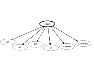
In statistics, naive Bayes classifiers are a family of linear "probabilistic classifiers" which assumes that the features are conditionally independent, given the target class. The strength (naivety) of this assumption is what gives the classifier its name. These classifiers are among the simplest Bayesian network models.

In statistics, the standard score is the number of standard deviations by which the value of a raw score is above or below the mean value of what is being observed or measured. Raw scores above the mean have positive standard scores, while those below the mean have negative standard scores.
The curse of dimensionality refers to various phenomena that arise when analyzing and organizing data in high-dimensional spaces that do not occur in low-dimensional settings such as the three-dimensional physical space of everyday experience. The expression was coined by Richard E. Bellman when considering problems in dynamic programming. The curse generally refers to issues that arise when the number of datapoints is small relative to the intrinsic dimension of the data.
Stochastic gradient descent is an iterative method for optimizing an objective function with suitable smoothness properties. It can be regarded as a stochastic approximation of gradient descent optimization, since it replaces the actual gradient by an estimate thereof. Especially in high-dimensional optimization problems this reduces the very high computational burden, achieving faster iterations in exchange for a lower convergence rate.
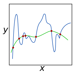
In mathematics, statistics, finance, computer science, particularly in machine learning and inverse problems, regularization is a process that changes the result answer to be "simpler". It is often used to obtain results for ill-posed problems or to prevent overfitting.
Least mean squares (LMS) algorithms are a class of adaptive filter used to mimic a desired filter by finding the filter coefficients that relate to producing the least mean square of the error signal. It is a stochastic gradient descent method in that the filter is only adapted based on the error at the current time. It was invented in 1960 by Stanford University professor Bernard Widrow and his first Ph.D. student, Ted Hoff, based on their research in single-layer neural networks (ADALINE). Specifically, they used gradient descent to train ADALINE to recognize patterns, and called the algorithm "delta rule". They then applied the rule to filters, resulting in the LMS algorithm.
In image processing, normalization is a process that changes the range of pixel intensity values. Applications include photographs with poor contrast due to glare, for example. Normalization is sometimes called contrast stretching or histogram stretching. In more general fields of data processing, such as digital signal processing, it is referred to as dynamic range expansion.
The softmax function, also known as softargmax or normalized exponential function, converts a vector of K real numbers into a probability distribution of K possible outcomes. It is a generalization of the logistic function to multiple dimensions, and used in multinomial logistic regression. The softmax function is often used as the last activation function of a neural network to normalize the output of a network to a probability distribution over predicted output classes, based on Luce's choice axiom.
The root-mean-square deviation (RMSD) or root-mean-square error (RMSE) is either one of two closely related and frequently used measures of the differences between true or predicted values on the one hand and observed values or an estimator on the other.
The rescaled range is a statistical measure of the variability of a time series introduced by the British hydrologist Harold Edwin Hurst (1880–1978). Its purpose is to provide an assessment of how the apparent variability of a series changes with the length of the time-period being considered.
Mean shift is a non-parametric feature-space mathematical analysis technique for locating the maxima of a density function, a so-called mode-seeking algorithm. Application domains include cluster analysis in computer vision and image processing.
BIRCH is an unsupervised data mining algorithm used to perform hierarchical clustering over particularly large data-sets. With modifications it can also be used to accelerate k-means clustering and Gaussian mixture modeling with the expectation–maximization algorithm. An advantage of BIRCH is its ability to incrementally and dynamically cluster incoming, multi-dimensional metric data points in an attempt to produce the best quality clustering for a given set of resources. In most cases, BIRCH only requires a single scan of the database.
Silhouette refers to a method of interpretation and validation of consistency within clusters of data. The technique provides a succinct graphical representation of how well each object has been classified. It was proposed by Belgian statistician Peter Rousseeuw in 1987.

In machine learning, Manifold regularization is a technique for using the shape of a dataset to constrain the functions that should be learned on that dataset. In many machine learning problems, the data to be learned do not cover the entire input space. For example, a facial recognition system may not need to classify any possible image, but only the subset of images that contain faces. The technique of manifold learning assumes that the relevant subset of data comes from a manifold, a mathematical structure with useful properties. The technique also assumes that the function to be learned is smooth: data with different labels are not likely to be close together, and so the labeling function should not change quickly in areas where there are likely to be many data points. Because of this assumption, a manifold regularization algorithm can use unlabeled data to inform where the learned function is allowed to change quickly and where it is not, using an extension of the technique of Tikhonov regularization. Manifold regularization algorithms can extend supervised learning algorithms in semi-supervised learning and transductive learning settings, where unlabeled data are available. The technique has been used for applications including medical imaging, geographical imaging, and object recognition.
Batch normalization is a method used to make training of artificial neural networks faster and more stable through normalization of the layers' inputs by re-centering and re-scaling. It was proposed by Sergey Ioffe and Christian Szegedy in 2015.


