It is a widely used effect in graphics software, typically to reduce image noise and reduce detail. The visual effect of this blurring technique is a smooth blur resembling that of viewing the image through a translucent screen, distinctly different from the bokeh effect produced by an out-of-focus lens or the shadow of an object under usual illumination.
Mathematically, applying a Gaussian blur to an image is the same as convolving the image with a Gaussian function. This is also known as a two-dimensional Weierstrass transform. By contrast, convolving by a circle (i.e., a circular box blur) would more accurately reproduce the bokeh effect.
Since the Fourier transform of a Gaussian is another Gaussian, applying a Gaussian blur has the effect of reducing the image's high-frequency components; a Gaussian blur is thus a low-pass filter.
A halftone print rendered smooth through Gaussian blur
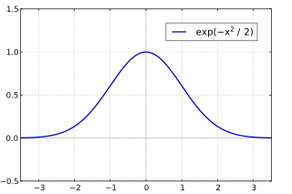
The Gaussian blur is a type of image-blurring filter that uses a Gaussian function (which also expresses the normal distribution in statistics) for calculating the transformation to apply to each pixel in the image. The formula of a Gaussian function in one dimension is
In two dimensions, it is the product of two such Gaussian functions, one in each dimension:[1][2][3] where x is the distance from the origin in the horizontal axis, y is the distance from the origin in the vertical axis, and σ is the standard deviation of the Gaussian distribution. It is important to note that the origin on these axes are at the center (0, 0). When applied in two dimensions, this formula produces a surface whose contours are concentric circles with a Gaussian distribution from the center point.
Values from this distribution are used to build a convolution matrix which is applied to the original image. This convolution process is illustrated visually in the figure on the right. Each pixel's new value is set to a weighted average of that pixel's neighborhood. The original pixel's value receives the heaviest weight (having the highest Gaussian value) and neighboring pixels receive smaller weights as their distance to the original pixel increases. This results in a blur that preserves boundaries and edges better than other, more uniform blurring filters; see also scale space implementation.
In theory, the Gaussian function at every point on the image will be non-zero, meaning that the entire image would need to be included in the calculations for each pixel. In practice, when computing a discrete approximation of the Gaussian function, pixels at a distance of more than 3σhave a small enough influence to be considered effectively zero. Thus contributions from pixels outside that range can be ignored. Typically, an image processing program need only calculate a matrix with dimensions × (where is the ceiling function) to ensure a result sufficiently close to that obtained by the entire Gaussian distribution.
In addition to being circularly symmetric, the Gaussian blur can be applied to a two-dimensional image as two independent one-dimensional calculations, and so is termed a separable filter. That is, the effect of applying the two-dimensional matrix can also be achieved by applying a series of single-dimensional Gaussian matrices in the horizontal direction, then repeating the process in the vertical direction. In computational terms, this is a useful property, since the calculation can be performed in time (where h is height and w is width; see Big O notation), as opposed to for a non-separable kernel.
Applying successive Gaussian blurs to an image has the same effect as applying a single, larger Gaussian blur, whose radius is the square root of the sum of the squares of the blur radii that were actually applied. For example, applying successive Gaussian blurs with radii of 6 and 8 gives the same results as applying a single Gaussian blur of radius 10, since . Because of this relationship, processing time cannot be saved by simulating a Gaussian blur with successive, smaller blurs — the time required will be at least as great as performing the single large blur.
Two downscaled images of the Flag of the Commonwealth of Nations. Before downscaling, a Gaussian blur was applied to the bottom image but not to the top image. The blur makes the image less sharp, but prevents the formation of moiré pattern aliasing artifacts.
Gaussian blurring is commonly used when reducing the size of an image. When downsampling an image, it is common to apply a low-pass filter to the image prior to resampling. This is to ensure that spurious high-frequency information does not appear in the downsampled image (aliasing). Gaussian blurs have nice properties, such as having no sharp edges, and thus do not introduce ringing into the filtered image.
Low-pass filter
This section needs expansion. You can help by adding to it. (March 2009)
Gaussian blur is a low-pass filter, attenuating high frequency signals.[3]
How much does a Gaussian filter with standard deviation smooth the picture? In other words, how much does it reduce the standard deviation of pixel values in the picture? Assume the grayscale pixel values have a standard deviation , then after applying the filter the reduced standard deviation can be approximated as[citation needed]
Sample Gaussian matrix
This sample matrix is produced by sampling the Gaussian filter kernel (with σ = 0.84089642) at the midpoints of each pixel and then normalizing. The center element (at [0, 0]) has the largest value, decreasing symmetrically as distance from the center increases. Since the filter kernel's origin is at the center, the matrix starts at and ends at where R equals the kernel radius.
The element 0.22508352 (the central one) is 1177 times larger than 0.00019117 which is just outside 3σ.
Implementation
A Gaussian blur effect is typically generated by convolving an image with an FIR kernel of Gaussian values, see [4] for an in-depth treatment.
In practice, it is best to take advantage of the Gaussian blur’s separable property by dividing the process into two passes. In the first pass, a one-dimensional kernel is used to blur the image in only the horizontal or vertical direction. In the second pass, the same one-dimensional kernel is used to blur in the remaining direction. The resulting effect is the same as convolving with a two-dimensional kernel in a single pass, but requires fewer calculations.
Discretization is typically achieved by sampling the Gaussian filter kernel at discrete points, normally at positions corresponding to the midpoints of each pixel. This reduces the computational cost but, for very small filter kernels, point sampling the Gaussian function with very few samples leads to a large error. In these cases, accuracy is maintained (at a slight computational cost) by integration of the Gaussian function over each pixel's area.[5]
When converting the Gaussian’s continuous values into the discrete values needed for a kernel, the sum of the values will be different from 1. This will cause a darkening or brightening of the image. To remedy this, the values can be normalized by dividing each term in the kernel by the sum of all terms in the kernel.
A much better and theoretically more well-founded approach is to instead perform the smoothing with the discrete analogue of the Gaussian kernel,[6] which possesses similar properties over a discrete domain as makes the continuous Gaussian kernel special over a continuous domain, for example, the kernel corresponding to the solution of a diffusion equation describing a spatial smoothing process, obeying a semi-group property over additions of the variance of the kernel, or describing the effect of Brownian motion over a spatial domain, and with the sum of its values being exactly equal to 1. For a more detailed description about the discrete analogue of the Gaussian kernel, see the article on scale-space implementation and.[6]
The efficiency of FIR breaks down for high sigmas. Alternatives to the FIR filter exist. These include the very fast multiple box blurs, the fast and accurate IIRDeriche edge detector, a "stack blur" based on the box blur, and more.[7]
Time-causal temporal smoothing
For processing pre-recorded temporal signals or video, the Gaussian kernel can also be used for smoothing over the temporal domain, since the data are pre-recorded and available in all directions. When processing temporal signals or video in real-time situations, the Gaussian kernel cannot, however, be used for temporal smoothing, since it would access data from the future, which obviously cannot be available. For temporal smoothing in real-time situations, one can instead use the temporal kernel referred to as the time-causal limit kernel,[8] which possesses similar properties in a time-causal situation (non-creation of new structures towards increasing scale and temporal scale covariance) as the Gaussian kernel obeys in the non-causal case. The time-causal limit kernel corresponds to convolution with an infinite number of truncated exponential kernels coupled in cascade, with specifically chosen time constants. For discrete data, this kernel can often be numerically well approximated by a small set of first-order recursive filters coupled in cascade, see [8] for further details.
Common uses
This shows how smoothing affects edge detection. With more smoothing, fewer edges are detected.
Edge detection
Gaussian smoothing is commonly used with edge detection. Most edge-detection algorithms are sensitive to noise; the 2-D Laplacian filter, built from a discretization of the Laplace operator, is highly sensitive to noisy environments.
Using a Gaussian Blur filter before edge detection aims to reduce the level of noise in the image, which improves the result of the following edge-detection algorithm. This approach is commonly referred to as Laplacian of Gaussian, or LoG filtering.[9]
Gaussian blur is automatically applied as part of the image post-processing of the photo by the camera software, leading to an irreversible loss of detail.[10][bettersourceneeded]
In mathematics, a Gaussian function, often simply referred to as a Gaussian, is a function of the base form and with parametric extension for arbitrary real constants a, b and non-zero c. It is named after the mathematician Carl Friedrich Gauss. The graph of a Gaussian is a characteristic symmetric "bell curve" shape. The parameter a is the height of the curve's peak, b is the position of the center of the peak, and c controls the width of the "bell".
Edge detection includes a variety of mathematical methods that aim at identifying edges, defined as curves in a digital image at which the image brightness changes sharply or, more formally, has discontinuities. The same problem of finding discontinuities in one-dimensional signals is known as step detection and the problem of finding signal discontinuities over time is known as change detection. Edge detection is a fundamental tool in image processing, machine vision and computer vision, particularly in the areas of feature detection and feature extraction.
The Canny edge detector is an edge detection operator that uses a multi-stage algorithm to detect a wide range of edges in images. It was developed by John F. Canny in 1986. Canny also produced a computational theory of edge detection explaining why the technique works.
The scale-invariant feature transform (SIFT) is a computer vision algorithm to detect, describe, and match local features in images, invented by David Lowe in 1999. Applications include object recognition, robotic mapping and navigation, image stitching, 3D modeling, gesture recognition, video tracking, individual identification of wildlife and match moving.
In image processing, a Gabor filter, named after Dennis Gabor, who first proposed it as a 1D filter. The Gabor filter was first generalized to 2D by Gösta Granlund, by adding a reference direction. The Gabor filter is a linear filter used for texture analysis, which essentially means that it analyzes whether there is any specific frequency content in the image in specific directions in a localized region around the point or region of analysis. Frequency and orientation representations of Gabor filters are claimed by many contemporary vision scientists to be similar to those of the human visual system. They have been found to be particularly appropriate for texture representation and discrimination. In the spatial domain, a 2D Gabor filter is a Gaussian kernel function modulated by a sinusoidal plane wave.
Scale-space theory is a framework for multi-scale signal representation developed by the computer vision, image processing and signal processing communities with complementary motivations from physics and biological vision. It is a formal theory for handling image structures at different scales, by representing an image as a one-parameter family of smoothed images, the scale-space representation, parametrized by the size of the smoothing kernel used for suppressing fine-scale structures. The parameter in this family is referred to as the scale parameter, with the interpretation that image structures of spatial size smaller than about have largely been smoothed away in the scale-space level at scale .
Lanczos filtering and Lanczos resampling are two applications of a certain mathematical formula. It can be used as a low-pass filter or used to smoothly interpolate the value of a digital signal between its samples. In the latter case, it maps each sample of the given signal to a translated and scaled copy of the Lanczos kernel, which is a sinc function windowed by the central lobe of a second, longer, sinc function. The sum of these translated and scaled kernels is then evaluated at the desired points.
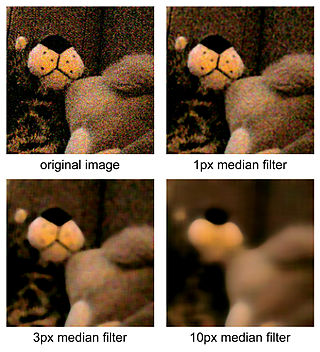
The median filter is a non-linear digital filtering technique, often used to remove noise from an image or signal. Such noise reduction is a typical pre-processing step to improve the results of later processing. Median filtering is very widely used in digital image processing because, under certain conditions, it preserves edges while removing noise, also having applications in signal processing.
The structural similarityindex measure (SSIM) is a method for predicting the perceived quality of digital television and cinematic pictures, as well as other kinds of digital images and videos. It is also used for measuring the similarity between two images. The SSIM index is a full reference metric; in other words, the measurement or prediction of image quality is based on an initial uncompressed or distortion-free image as reference.
In imaging science, difference of Gaussians (DoG) is a feature enhancement algorithm that involves the subtraction of one Gaussian blurred version of an original image from another, less blurred version of the original. In the simple case of grayscale images, the blurred images are obtained by convolving the original grayscale images with Gaussian kernels having differing width. Blurring an image using a Gaussian kernel suppresses only high-frequency spatial information. Subtracting one image from the other preserves spatial information that lies between the range of frequencies that are preserved in the two blurred images. Thus, the DoG is a spatial band-pass filter that attenuates frequencies in the original grayscale image that are far from the band center.
The Gabor transform, named after Dennis Gabor, is a special case of the short-time Fourier transform. It is used to determine the sinusoidal frequency and phase content of local sections of a signal as it changes over time. The function to be transformed is first multiplied by a Gaussian function, which can be regarded as a window function, and the resulting function is then transformed with a Fourier transform to derive the time-frequency analysis. The window function means that the signal near the time being analyzed will have higher weight. The Gabor transform of a signal x(t) is defined by this formula:
The scale space representation of a signal obtained by Gaussian smoothing satisfies a number of special properties, scale-space axioms, which make it into a special form of multi-scale representation. There are, however, also other types of "multi-scale approaches" in the areas of computer vision, image processing and signal processing, in particular the notion of wavelets. The purpose of this article is to describe a few of these approaches:
In electronics and signal processing, mainly in digital signal processing, a Gaussian filter is a filter whose impulse response is a Gaussian function. Gaussian filters have the properties of having no overshoot to a step function input while minimizing the rise and fall time. This behavior is closely connected to the fact that the Gaussian filter has the minimum possible group delay. A Gaussian filter will have the best combination of suppression of high frequencies while also minimizing spatial spread, being the critical point of the uncertainty principle. These properties are important in areas such as oscilloscopes and digital telecommunication systems.
Affine shape adaptation is a methodology for iteratively adapting the shape of the smoothing kernels in an affine group of smoothing kernels to the local image structure in neighbourhood region of a specific image point. Equivalently, affine shape adaptation can be accomplished by iteratively warping a local image patch with affine transformations while applying a rotationally symmetric filter to the warped image patches. Provided that this iterative process converges, the resulting fixed point will be affine invariant. In the area of computer vision, this idea has been used for defining affine invariant interest point operators as well as affine invariant texture analysis methods.
In mathematics, the structure tensor, also referred to as the second-moment matrix, is a matrix derived from the gradient of a function. It describes the distribution of the gradient in a specified neighborhood around a point and makes the information invariant to the observing coordinates. The structure tensor is often used in image processing and computer vision.
Mean shift is a non-parametric feature-space mathematical analysis technique for locating the maxima of a density function, a so-called mode-seeking algorithm. Application domains include cluster analysis in computer vision and image processing.
In computer vision, speeded up robust features (SURF) is a local feature detector and descriptor, with patented applications. It can be used for tasks such as object recognition, image registration, classification, or 3D reconstruction. It is partly inspired by the scale-invariant feature transform (SIFT) descriptor. The standard version of SURF is several times faster than SIFT and claimed by its authors to be more robust against different image transformations than SIFT.
In the fields of computer vision and image analysis, the Harris affine region detector belongs to the category of feature detection. Feature detection is a preprocessing step of several algorithms that rely on identifying characteristic points or interest points so to make correspondences between images, recognize textures, categorize objects or build panoramas.
In image processing and computer vision, anisotropic diffusion, also called Perona–Malik diffusion, is a technique aiming at reducing image noise without removing significant parts of the image content, typically edges, lines or other details that are important for the interpretation of the image. Anisotropic diffusion resembles the process that creates a scale space, where an image generates a parameterized family of successively more and more blurred images based on a diffusion process. Each of the resulting images in this family are given as a convolution between the image and a 2D isotropic Gaussian filter, where the width of the filter increases with the parameter. This diffusion process is a linear and space-invariant transformation of the original image. Anisotropic diffusion is a generalization of this diffusion process: it produces a family of parameterized images, but each resulting image is a combination between the original image and a filter that depends on the local content of the original image. As a consequence, anisotropic diffusion is a non-linear and space-variant transformation of the original image.
Kernel methods are a well-established tool to analyze the relationship between input data and the corresponding output of a function. Kernels encapsulate the properties of functions in a computationally efficient way and allow algorithms to easily swap functions of varying complexity.
This page is based on this Wikipedia article Text is available under the CC BY-SA 4.0 license; additional terms may apply. Images, videos and audio are available under their respective licenses.