
Pink noise, 1⁄f noise or fractal noise is a signal or process with a frequency spectrum such that the power spectral density is inversely proportional to the frequency of the signal. In pink noise, each octave interval carries an equal amount of noise energy.
Rayleigh fading is a statistical model for the effect of a propagation environment on a radio signal, such as that used by wireless devices.
Rician fading or Ricean fading is a stochastic model for radio propagation anomaly caused by partial cancellation of a radio signal by itself — the signal arrives at the receiver by several different paths, and at least one of the paths is changing. Rician fading occurs when one of the paths, typically a line of sight signal or some strong reflection signals, is much stronger than the others. In Rician fading, the amplitude gain is characterized by a Rician distribution.

A sensor array is a group of sensors, usually deployed in a certain geometry pattern, used for collecting and processing electromagnetic or acoustic signals. The advantage of using a sensor array over using a single sensor lies in the fact that an array adds new dimensions to the observation, helping to estimate more parameters and improve the estimation performance. For example an array of radio antenna elements used for beamforming can increase antenna gain in the direction of the signal while decreasing the gain in other directions, i.e., increasing signal-to-noise ratio (SNR) by amplifying the signal coherently. Another example of sensor array application is to estimate the direction of arrival of impinging electromagnetic waves. The related processing method is called array signal processing. A third examples includes chemical sensor arrays, which utilize multiple chemical sensors for fingerprint detection in complex mixtures or sensing environments. Application examples of array signal processing include radar/sonar, wireless communications, seismology, machine condition monitoring, astronomical observations fault diagnosis, etc.
In signal processing, a matched filter is obtained by correlating a known delayed signal, or template, with an unknown signal to detect the presence of the template in the unknown signal. This is equivalent to convolving the unknown signal with a conjugated time-reversed version of the template. The matched filter is the optimal linear filter for maximizing the signal-to-noise ratio (SNR) in the presence of additive stochastic noise.
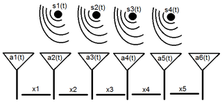
Array processing is a wide area of research in the field of signal processing that extends from the simplest form of 1 dimensional line arrays to 2 and 3 dimensional array geometries. Array structure can be defined as a set of sensors that are spatially separated, e.g. radio antenna and seismic arrays. The sensors used for a specific problem may vary widely, for example microphones, accelerometers and telescopes. However, many similarities exist, the most fundamental of which may be an assumption of wave propagation. Wave propagation means there is a systemic relationship between the signal received on spatially separated sensors. By creating a physical model of the wave propagation, or in machine learning applications a training data set, the relationships between the signals received on spatially separated sensors can be leveraged for many applications.
A stochastic differential equation (SDE) is a differential equation in which one or more of the terms is a stochastic process, resulting in a solution which is also a stochastic process. SDEs have many applications throughout pure mathematics and are used to model various behaviours of stochastic models such as stock prices, random growth models or physical systems that are subjected to thermal fluctuations.
In statistics and probability theory, a point process or point field is a collection of mathematical points randomly located on a mathematical space such as the real line or Euclidean space. Point processes can be used for spatial data analysis, which is of interest in such diverse disciplines as forestry, plant ecology, epidemiology, geography, seismology, materials science, astronomy, telecommunications, computational neuroscience, economics and others.
The log-distance path loss model is a radio propagation model that predicts the path loss a signal encounters inside a building or densely populated areas over distance.
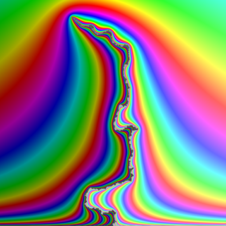
In probability theory, the Schramm–Loewner evolution with parameter κ, also known as stochastic Loewner evolution (SLEκ), is a family of random planar curves that have been proven to be the scaling limit of a variety of two-dimensional lattice models in statistical mechanics. Given a parameter κ and a domain in the complex plane U, it gives a family of random curves in U, with κ controlling how much the curve turns. There are two main variants of SLE, chordal SLE which gives a family of random curves from two fixed boundary points, and radial SLE, which gives a family of random curves from a fixed boundary point to a fixed interior point. These curves are defined to satisfy conformal invariance and a domain Markov property.
Cooperative diversity is a cooperative multiple antenna technique for improving or maximising total network channel capacities for any given set of bandwidths which exploits user diversity by decoding the combined signal of the relayed signal and the direct signal in wireless multihop networks. A conventional single hop system uses direct transmission where a receiver decodes the information only based on the direct signal while regarding the relayed signal as interference, whereas the cooperative diversity considers the other signal as contribution. That is, cooperative diversity decodes the information from the combination of two signals. Hence, it can be seen that cooperative diversity is an antenna diversity that uses distributed antennas belonging to each node in a wireless network. Note that user cooperation is another definition of cooperative diversity. User cooperation considers an additional fact that each user relays the other user's signal while cooperative diversity can be also achieved by multi-hop relay networking systems.
In mathematics, stochastic geometry is the study of random spatial patterns. At the heart of the subject lies the study of random point patterns. This leads to the theory of spatial point processes, hence notions of Palm conditioning, which extend to the more abstract setting of random measures.
In probability theory, a Laplace functional refers to one of two possible mathematical functions of functions or, more precisely, functionals that serve as mathematical tools for studying either point processes or concentration of measure properties of metric spaces. One type of Laplace functional, also known as a characteristic functional is defined in relation to a point process, which can be interpreted as random counting measures, and has applications in characterizing and deriving results on point processes. Its definition is analogous to a characteristic function for a random variable.
In mathematics, a determinantal point process is a stochastic point process, the probability distribution of which is characterized as a determinant of some function. Such processes arise as important tools in random matrix theory, combinatorics, physics, and wireless network modeling.
In probability theory and statistics, Campbell's theorem or the Campbell–Hardy theorem is either a particular equation or set of results relating to the expectation of a function summed over a point process to an integral involving the mean measure of the point process, which allows for the calculation of expected value and variance of the random sum. One version of the theorem, also known as Campbell's formula, entails an integral equation for the aforementioned sum over a general point process, and not necessarily a Poisson point process. There also exist equations involving moment measures and factorial moment measures that are considered versions of Campbell's formula. All these results are employed in probability and statistics with a particular importance in the theory of point processes and queueing theory as well as the related fields stochastic geometry, continuum percolation theory, and spatial statistics.
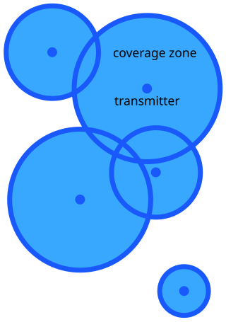
In mathematics and probability theory, continuum percolation theory is a branch of mathematics that extends discrete percolation theory to continuous space. More specifically, the underlying points of discrete percolation form types of lattices whereas the underlying points of continuum percolation are often randomly positioned in some continuous space and form a type of point process. For each point, a random shape is frequently placed on it and the shapes overlap each with other to form clumps or components. As in discrete percolation, a common research focus of continuum percolation is studying the conditions of occurrence for infinite or giant components. Other shared concepts and analysis techniques exist in these two types of percolation theory as well as the study of random graphs and random geometric graphs.
In mathematics and telecommunications, stochastic geometry models of wireless networks refer to mathematical models based on stochastic geometry that are designed to represent aspects of wireless networks. The related research consists of analyzing these models with the aim of better understanding wireless communication networks in order to predict and control various network performance metrics. The models require using techniques from stochastic geometry and related fields including point processes, spatial statistics, geometric probability, percolation theory, as well as methods from more general mathematical disciplines such as geometry, probability theory, stochastic processes, queueing theory, information theory, and Fourier analysis.
In probability and statistics, point process notation comprises the range of mathematical notation used to symbolically represent random objects known as point processes, which are used in related fields such as stochastic geometry, spatial statistics and continuum percolation theory and frequently serve as mathematical models of random phenomena, representable as points, in time, space or both.

In probability, statistics and related fields, a Poisson point process is a type of random mathematical object that consists of points randomly located on a mathematical space with the essential feature that the points occur independently of one another. The Poisson point process is often called simply the Poisson process, but it is also called a Poisson random measure, Poisson random point field or Poisson point field. This point process has convenient mathematical properties, which has led to its being frequently defined in Euclidean space and used as a mathematical model for seemingly random processes in numerous disciplines such as astronomy, biology, ecology, geology, seismology, physics, economics, image processing, and telecommunications.
In radio propagation, two-wave with diffuse power (TWDP) fading is a model that explains why a signal strengthens or weakens at certain locations or times. TWDP models fading due to the interference of two strong radio signals and numerous smaller, diffuse signals.


