Reassignment method

Reassigned spectral surface for the onset of an acoustic bass tone having a sharp pluck and a fundamental frequency of approximately 73.4 Hz. Sharp spectral ridges representing the harmonics are evident, as is the abrupt onset of the tone. The spectrogram was computed using a 65.7 ms Kaiser window with a shaping parameter of 12.

The method of reassignment is a technique for sharpening a time-frequency representation (e.g. spectrogram or the short-time Fourier transform) by mapping the data to time-frequency coordinates that are nearer to the true region of support of the analyzed signal. The method has been independently introduced by several parties under various names, including method of reassignment, remapping, time-frequency reassignment, and modified moving-window method. ^[1] The method of reassignment sharpens blurry time-frequency data by relocating the data according to local estimates of instantaneous frequency and group delay. This mapping to reassigned time-frequency coordinates is very precise for signals that are separable in time and frequency with respect to the analysis window.

Introduction

Many signals of interest have a distribution of energy that varies in time and frequency. For example, any sound signal having a beginning or an end has an energy distribution that varies in time, and most sounds exhibit considerable variation in both time and frequency over their duration. Time-frequency representations are commonly used to analyze or characterize such signals. They map the one-dimensional time-domain signal into a two-dimensional function of time and frequency. A time-frequency representation describes the variation of spectral energy distribution over time, much as a musical score describes the variation of musical pitch over time.

In audio signal analysis, the spectrogram is the most commonly used time-frequency representation, probably because it is well understood, and immune to so-called "cross-terms" that sometimes make other time-frequency representations difficult to interpret. But the windowing operation required in spectrogram computation introduces an unsavory tradeoff between time resolution and frequency resolution, so spectrograms provide a time-frequency representation that is blurred in time, in frequency, or in both dimensions. The method of time-frequency reassignment is a technique for refocussing time-frequency data in a blurred representation like the spectrogram by mapping the data to time-frequency coordinates that are nearer to the true region of support of the analyzed signal. ^[2]

The spectrogram as a time-frequency representation

Main article: Spectrogram

One of the best-known time-frequency representations is the spectrogram, defined as the squared magnitude of the short-time Fourier transform. Though the short-time phase spectrum is known to contain important temporal information about the signal, this information is difficult to interpret, so typically, only the short-time magnitude spectrum is considered in short-time spectral analysis. ^[2]

As a time-frequency representation, the spectrogram has relatively poor resolution. Time and frequency resolution are governed by the choice of analysis window and greater concentration in one domain is accompanied by greater smearing in the other. ^[2]

A time-frequency representation having improved resolution, relative to the spectrogram, is the Wigner–Ville distribution, which may be interpreted as a short-time Fourier transform with a window function that is perfectly matched to the signal. The Wigner–Ville distribution is highly concentrated in time and frequency, but it is also highly nonlinear and non-local. Consequently, this distribution is very sensitive to noise, and generates cross-components that often mask the components of interest, making it difficult to extract useful information concerning the distribution of energy in multi-component signals. ^[2]

Cohen's class of bilinear time-frequency representations is a class of "smoothed" Wigner–Ville distributions, employing a smoothing kernel that can reduce sensitivity of the distribution to noise and suppresses cross-components, at the expense of smearing the distribution in time and frequency. This smearing causes the distribution to be non-zero in regions where the true Wigner–Ville distribution shows no energy. ^[2]

The spectrogram is a member of Cohen's class. It is a smoothed Wigner–Ville distribution with the smoothing kernel equal to the Wigner–Ville distribution of the analysis window. The method of reassignment smooths the Wigner–Ville distribution, but then refocuses the distribution back to the true regions of support of the signal components. The method has been shown to reduce time and frequency smearing of any member of Cohen's class. ^{[2] [3]} In the case of the reassigned spectrogram, the short-time phase spectrum is used to correct the nominal time and frequency coordinates of the spectral data, and map it back nearer to the true regions of support of the analyzed signal.

The method of reassignment

Pioneering work on the method of reassignment was published by Kodera, Gendrin, and de Villedary under the name of Modified Moving Window Method. ^[4] Their technique enhances the resolution in time and frequency of the classical Moving Window Method (equivalent to the spectrogram) by assigning to each data point a new time-frequency coordinate that better-reflects the distribution of energy in the analyzed signal. ^{[4] : 67}

In the classical moving window method, a time-domain signal, ${\displaystyle x(t)}$ is decomposed into a set of coefficients, ${\displaystyle \epsilon (t,\omega )}$, based on a set of elementary signals, ${\displaystyle h_{\omega }(t)}$, defined ^{[4] : 73}

${\displaystyle h_{\omega }(t)=h(t)e^{j\omega t}}$

where ${\displaystyle h(t)}$ is a (real-valued) lowpass kernel function, like the window function in the short-time Fourier transform. The coefficients in this decomposition are defined

${\displaystyle {\begin{aligned}\epsilon (t,\omega )&=\int x(\tau )h(t-\tau )e^{-j\omega \left[\tau -t\right]}d\tau \\&=e^{j\omega t}\int x(\tau )h(t-\tau )e^{-j\omega \tau }d\tau \\&=e^{j\omega t}X(t,\omega )\\&=X_{t}(\omega )\\&=M_{t}(\omega )e^{j\phi _{\tau }(\omega )}\end{aligned}}}$

where ${\displaystyle M_{t}(\omega )}$ is the magnitude, and ${\displaystyle \phi _{\tau }(\omega )}$ the phase, of ${\displaystyle X_{t}(\omega )}$, the Fourier transform of the signal ${\displaystyle x(t)}$ shifted in time by ${\displaystyle t}$ and windowed by ${\displaystyle h(t)}$. ^{[5] : 4}

${\displaystyle x(t)}$ can be reconstructed from the moving window coefficients by ^{[5] : 8}

${\displaystyle {\begin{aligned}x(t)&=\iint X_{\tau }(\omega )h_{\omega }^{*}(\tau -t)d\omega d\tau \\&=\iint X_{\tau }(\omega )h(\tau -t)e^{-j\omega \left[\tau -t\right]}d\omega d\tau \\&=\iint M_{\tau }(\omega )e^{j\phi _{\tau }(\omega )}h(\tau -t)e^{-j\omega \left[\tau -t\right]}d\omega d\tau \\&=\iint M_{\tau }(\omega )h(\tau -t)e^{j\left[\phi _{\tau }(\omega )-\omega \tau +\omega t\right]}d\omega d\tau \end{aligned}}}$

For signals having magnitude spectra, ${\displaystyle M(t,\omega )}$, whose time variation is slow relative to the phase variation, the maximum contribution to the reconstruction integral comes from the vicinity of the point ${\displaystyle t,\omega }$ satisfying the phase stationarity condition ^{[4] : 74}

${\displaystyle {\begin{aligned}{\frac {\partial }{\partial \omega }}\left[\phi _{\tau }(\omega )-\omega \tau +\omega t\right]&=0\\{\frac {\partial }{\partial \tau }}\left[\phi _{\tau }(\omega )-\omega \tau +\omega t\right]&=0\end{aligned}}}$

or equivalently, around the point ${\displaystyle {\hat {t}},{\hat {\omega }}}$ defined by ^{[4] : 74}

${\displaystyle {\begin{aligned}{\hat {t}}(\tau ,\omega )&=\tau -{\frac {\partial \phi _{\tau }(\omega )}{\partial \omega }}=-{\frac {\partial \phi (\tau ,\omega )}{\partial \omega }}\\{\hat {\omega }}(\tau ,\omega )&={\frac {\partial \phi _{\tau }(\omega )}{\partial \tau }}=\omega +{\frac {\partial \phi (\tau ,\omega )}{\partial \tau }}\end{aligned}}}$

This phenomenon is known in such fields as optics as the principle of stationary phase, which states that for periodic or quasi-periodic signals, the variation of the Fourier phase spectrum not attributable to periodic oscillation is slow with respect to time in the vicinity of the frequency of oscillation, and in surrounding regions the variation is relatively rapid. Analogously, for impulsive signals, that are concentrated in time, the variation of the phase spectrum is slow with respect to frequency near the time of the impulse, and in surrounding regions the variation is relatively rapid. ^{[4] : 73}

In reconstruction, positive and negative contributions to the synthesized waveform cancel, due to destructive interference, in frequency regions of rapid phase variation. Only regions of slow phase variation (stationary phase) will contribute significantly to the reconstruction, and the maximum contribution (center of gravity) occurs at the point where the phase is changing most slowly with respect to time and frequency. ^{[4] : 71}

The time-frequency coordinates thus computed are equal to the local group delay, ${\displaystyle {\hat {t}}_{g}(t,\omega ),}$ and local instantaneous frequency, ${\displaystyle {\hat {\omega }}_{i}(t,\omega ),}$ and are computed from the phase of the short-time Fourier transform, which is normally ignored when constructing the spectrogram. These quantities are local in the sense that they represent a windowed and filtered signal that is localized in time and frequency, and are not global properties of the signal under analysis. ^{[4] : 70}

The modified moving window method, or method of reassignment, changes (reassigns) the point of attribution of ${\displaystyle \epsilon (t,\omega )}$ to this point of maximum contribution ${\displaystyle {\hat {t}}(t,\omega ),{\hat {\omega }}(t,\omega )}$, rather than to the point ${\displaystyle t,\omega }$ at which it is computed. This point is sometimes called the center of gravity of the distribution, by way of analogy to a mass distribution. This analogy is a useful reminder that the attribution of spectral energy to the center of gravity of its distribution only makes sense when there is energy to attribute, so the method of reassignment has no meaning at points where the spectrogram is zero-valued. ^[2]

Efficient computation of reassigned times and frequencies

In digital signal processing, it is most common to sample the time and frequency domains. The discrete Fourier transform is used to compute samples ${\displaystyle X(k)}$ of the Fourier transform from samples ${\displaystyle x(n)}$ of a time domain signal. The reassignment operations proposed by Kodera et al. cannot be applied directly to the discrete short-time Fourier transform data, because partial derivatives cannot be computed directly on data that is discrete in time and frequency, and it has been suggested that this difficulty has been the primary barrier to wider use of the method of reassignment.

It is possible to approximate the partial derivatives using finite differences. For example, the phase spectrum can be evaluated at two nearby times, and the partial derivative with respect to time be approximated as the difference between the two values divided by the time difference, as in

${\displaystyle {\begin{aligned}{\frac {\partial \phi (t,\omega )}{\partial t}}&\approx {\frac {1}{\Delta t}}\left[\phi \left(t+{\frac {\Delta t}{2}},\omega \right)-\phi \left(t-{\frac {\Delta t}{2}},\omega \right)\right]\\{\frac {\partial \phi (t,\omega )}{\partial \omega }}&\approx {\frac {1}{\Delta \omega }}\left[\phi \left(t,\omega +{\frac {\Delta \omega }{2}}\right)-\phi \left(t,\omega -{\frac {\Delta \omega }{2}}\right)\right]\end{aligned}}}$

For sufficiently small values of ${\displaystyle \Delta t}$ and ${\displaystyle \Delta \omega ,}$ and provided that the phase difference is appropriately "unwrapped", this finite-difference method yields good approximations to the partial derivatives of phase, because in regions of the spectrum in which the evolution of the phase is dominated by rotation due to sinusoidal oscillation of a single, nearby component, the phase is a linear function.

Independently of Kodera et al., Nelson arrived at a similar method for improving the time-frequency precision of short-time spectral data from partial derivatives of the short-time phase spectrum. ^[6] It is easily shown that Nelson's cross spectral surfaces compute an approximation of the derivatives that is equivalent to the finite differences method.

Auger and Flandrin showed that the method of reassignment, proposed in the context of the spectrogram by Kodera et al., could be extended to any member of Cohen's class of time-frequency representations by generalizing the reassignment operations to

${\displaystyle {\begin{aligned}{\hat {t}}(t,\omega )&=t-{\frac {\iint \tau \cdot W_{x}(t-\tau ,\omega -\nu )\cdot \Phi (\tau ,\nu )d\tau d\nu }{\iint W_{x}\left(t-\tau ,\omega -\nu \right)\cdot \Phi (\tau ,\nu )d\tau d\nu }}\\{\hat {\omega }}(t,\omega )&=\omega -{\frac {\iint \nu \cdot W_{x}(t-\tau ,\omega -\nu )\cdot \Phi (\tau ,\nu )d\tau d\nu }{\iint W_{x}(t-\tau ,\omega -\nu )\cdot \Phi (\tau ,\nu )d\tau d\nu }}\end{aligned}}}$

where ${\displaystyle W_{x}(t,\omega )}$ is the Wigner–Ville distribution of ${\displaystyle x(t)}$, and ${\displaystyle \Phi (t,\omega )}$ is the kernel function that defines the distribution. They further described an efficient method for computing the times and frequencies for the reassigned spectrogram efficiently and accurately without explicitly computing the partial derivatives of phase. ^[2]

In the case of the spectrogram, the reassignment operations can be computed by

${\displaystyle {\begin{aligned}{\hat {t}}(t,\omega )&=t-\Re \left\{{\frac {X_{{\mathcal {T}}h}(t,\omega )\cdot X^{*}(t,\omega )}{|X(t,\omega )|^{2}}}\right\}\\{\hat {\omega }}(t,\omega )&=\omega +\Im \left\{{\frac {X_{{\mathcal {D}}h}(t,\omega )\cdot X^{*}(t,\omega )}{|X(t,\omega )|^{2}}}\right\}\end{aligned}}}$

where ${\displaystyle X(t,\omega )}$ is the short-time Fourier transform computed using an analysis window ${\displaystyle h(t),X_{{\mathcal {T}}h}(t,\omega )}$ is the short-time Fourier transform computed using a time-weighted analysis window ${\displaystyle h_{\mathcal {T}}(t)=t\cdot h(t)}$ and ${\displaystyle X_{{\mathcal {D}}h}(t,\omega )}$ is the short-time Fourier transform computed using a time-derivative analysis window ${\displaystyle h_{\mathcal {D}}(t)={\tfrac {d}{dt}}h(t)}$.

Using the auxiliary window functions ${\displaystyle h_{\mathcal {T}}(t)}$ and ${\displaystyle h_{\mathcal {D}}(t)}$, the reassignment operations can be computed at any time-frequency coordinate ${\displaystyle t,\omega }$ from an algebraic combination of three Fourier transforms evaluated at ${\displaystyle t,\omega }$. Since these algorithms operate only on short-time spectral data evaluated at a single time and frequency, and do not explicitly compute any derivatives, this gives an efficient method of computing the reassigned discrete short-time Fourier transform.

One constraint in this method of computation is that the ${\displaystyle |X(t,\omega )|^{2}}$ must be non-zero. This is not much of a restriction, since the reassignment operation itself implies that there is some energy to reassign, and has no meaning when the distribution is zero-valued.

Separability

The short-time Fourier transform can often be used to estimate the amplitudes and phases of the individual components in a multi-component signal, such as a quasi-harmonic musical instrument tone. Moreover, the time and frequency reassignment operations can be used to sharpen the representation by attributing the spectral energy reported by the short-time Fourier transform to the point that is the local center of gravity of the complex energy distribution. ^[7]

For a signal consisting of a single component, the instantaneous frequency can be estimated from the partial derivatives of phase of any short-time Fourier transform channel that passes the component. If the signal is to be decomposed into many components,

${\displaystyle x(t)=\sum _{n}A_{n}(t)e^{j\theta _{n}(t)}}$

and the instantaneous frequency of each component is defined as the derivative of its phase with respect to time, that is,

${\displaystyle \omega _{n}(t)={\frac {d\theta _{n}(t)}{dt}},}$

then the instantaneous frequency of each individual component can be computed from the phase of the response of a filter that passes that component, provided that no more than one component lies in the passband of the filter.

This is the property, in the frequency domain, that Nelson called separability ^[6] and is required of all signals so analyzed. If this property is not met, then the desired multi-component decomposition cannot be achieved, because the parameters of individual components cannot be estimated from the short-time Fourier transform. In such cases, a different analysis window must be chosen so that the separability criterion is satisfied.

If the components of a signal are separable in frequency with respect to a particular short-time spectral analysis window, then the output of each short-time Fourier transform filter is a filtered version of, at most, a single dominant (having significant energy) component, and so the derivative, with respect to time, of the phase of the ${\displaystyle X(t,\omega _{0})}$ is equal to the derivative with respect to time, of the phase of the dominant component at ${\displaystyle \omega _{0}.}$ Therefore, if a component, ${\displaystyle x_{n}(t),}$ having instantaneous frequency ${\displaystyle \omega _{n}(t)}$ is the dominant component in the vicinity of ${\displaystyle \omega _{0},}$ then the instantaneous frequency of that component can be computed from the phase of the short-time Fourier transform evaluated at ${\displaystyle \omega _{0}.}$ That is,

${\displaystyle {\begin{aligned}\omega _{n}(t)&={\frac {\partial }{\partial t}}\arg\{x_{n}(t)\}\\&={\frac {\partial }{\partial t}}\arg\{X(t,\omega _{0})\}\end{aligned}}}$

Just as each bandpass filter in the short-time Fourier transform filterbank may pass at most a single complex exponential component, two temporal events must be sufficiently separated in time that they do not lie in the same windowed segment of the input signal. This is the property of separability in the time domain, and is equivalent to requiring that the time between two events be greater than the length of the impulse response of the short-time Fourier transform filters, the span of non-zero samples in ${\displaystyle h(t).}$

• 
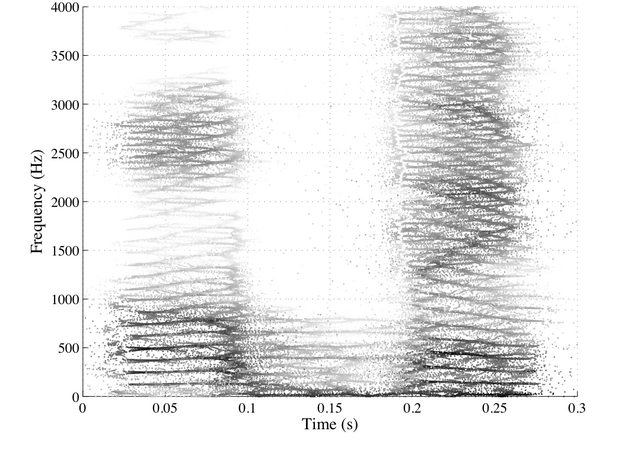
  Long-window reassigned spectrogram of the word "open", computed using a 54.4 ms Kaiser window with a shaping parameter of 9, emphasizing harmonics.
• 
  Short-window reassigned spectrogram of the word "open", computed using a 13.6 ms Kaiser window with a shaping parameter of 9, emphasizing formants and glottal pulses.

In general, there is an infinite number of equally valid decompositions for a multi-component signal. The separability property must be considered in the context of the desired decomposition. For example, in the analysis of a speech signal, an analysis window that is long relative to the time between glottal pulses is sufficient to separate harmonics, but the individual glottal pulses will be smeared, because many pulses are covered by each window (that is, the individual pulses are not separable, in time, by the chosen analysis window). An analysis window that is much shorter than the time between glottal pulses may resolve the glottal pulses, because no window spans more than one pulse, but the harmonic frequencies are smeared together, because the main lobe of the analysis window spectrum is wider than the spacing between the harmonics (that is, the harmonics are not separable, in frequency, by the chosen analysis window). ^{[6] : 2585}

Extensions

Consensus complex reassignmet

Gardner and Magnasco (2006) argues that the auditory nerves may use a form of the reassignment method to process sounds. These nerves are known for preserving timing (phase) information better than they do for magnitudes. The authors come up with a variation of reassignment with complex values (i.e. both phase and magnitude) and show that it produces sparse outputs like auditory nerves do. By running this reassignment with windows of different bandwidths (see discussion in the section above), a "consensus" that captures multiple kinds of signals is found, again like the auditory system. They argue that the algorithm is simple enough for neurons to implement. ^[8]

Synchrosqueezing transform

^[9]

References

1. Hainsworth, Stephen (2003). "Chapter 3: Reassignment methods". Techniques for the Automated Analysis of Musical Audio (PhD). University of Cambridge. CiteSeerX   10.1.1.5.9579 .
2. F. Auger & P. Flandrin (May 1995). "Improving the readability of time-frequency and time-scale representations by the reassignment method". IEEE Transactions on Signal Processing. 43 (5): 1068–1089. Bibcode:1995ITSP...43.1068A. CiteSeerX   10.1.1.646.794 . doi:10.1109/78.382394. S2CID   6336685.
3. P. Flandrin, F. Auger, and E. Chassande-Mottin, Time-frequency reassignment: From principles to algorithms, in Applications in Time-Frequency Signal Processing (A. Papandreou-Suppappola, ed.), ch. 5, pp. 179 – 203, CRC Press, 2003.
4. K. Kodera; R. Gendrin & C. de Villedary (Feb 1978). "Analysis of time-varying signals with small BT values". IEEE Transactions on Acoustics, Speech, and Signal Processing. 26 (1): 64–76. doi:10.1109/TASSP.1978.1163047.
5. Fitz, Kelly R.; Fulop, Sean A. (2009), A Unified Theory of Time-Frequency Reassignment, doi:10.48550/arXiv.0903.3080 – this preprint manuscript is written by a previous contributor to this Wikipedia article; see their contribution.
6. D. J. Nelson (Nov 2001). "Cross-spectral methods for processing speech". Journal of the Acoustical Society of America. 110 (5): 2575–2592. Bibcode:2001ASAJ..110.2575N. doi:10.1121/1.1402616. PMID   11757947.
7. K. Fitz, L. Haken, On the use of time-frequency reassignment in additve sound modeling, Journal of the Audio Engineering Society 50 (11) (2002) 879 – 893.
8. Gardner, Timothy J.; Magnasco, Marcelo O. (18 April 2006). "Sparse time-frequency representations". Proceedings of the National Academy of Sciences. 103 (16): 6094–6099. doi:10.1073/pnas.0601707103.
9. Meignen, Sylvain; Oberlin, Thomas; Pham, Duong-Hung (July 2019). "Synchrosqueezing transforms: From low- to high-frequency modulations and perspectives". Comptes Rendus Physique. 20 (5): 449–460. doi:10.1016/j.crhy.2019.07.001.

Further reading

• S. A. Fulop and K. Fitz, A spectrogram for the twenty-first century, Acoustics Today, vol. 2, no. 3, pp. 26–33, 2006.
• S. A. Fulop and K. Fitz, Algorithms for computing the time-corrected instantaneous frequency (reassigned) spectrogram, with applications, Journal of the Acoustical Society of America, vol. 119, pp. 360 – 371, Jan 2006.

External links

• TFTB — Time-Frequency ToolBox
• SPEAR - Sinusoidal Partial Editing Analysis and Resynthesis
• Loris - Open-source software for sound modeling and morphing
• SRA - A web-based research tool for spectral and roughness analysis of sound signals Archived 2019-11-18 at the Wayback Machine (supported by a Northwest Academic Computing Consortium grant to J. Middleton, Eastern Washington University)