
In physics, a dipole is an electromagnetic phenomenon which occurs in two ways:
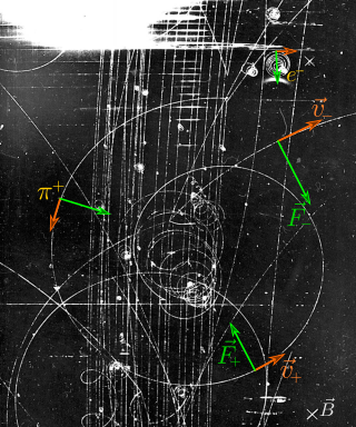
In physics, specifically in electromagnetism, the Lorentz force is the combination of electric and magnetic force on a point charge due to electromagnetic fields. A particle of charge q moving with a velocity v in an electric field E and a magnetic field B experiences a force of
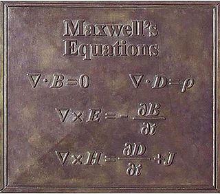
Maxwell's equations, or Maxwell–Heaviside equations, are a set of coupled partial differential equations that, together with the Lorentz force law, form the foundation of classical electromagnetism, classical optics, electric and magnetic circuits. The equations provide a mathematical model for electric, optical, and radio technologies, such as power generation, electric motors, wireless communication, lenses, radar, etc. They describe how electric and magnetic fields are generated by charges, currents, and changes of the fields. The equations are named after the physicist and mathematician James Clerk Maxwell, who, in 1861 and 1862, published an early form of the equations that included the Lorentz force law. Maxwell first used the equations to propose that light is an electromagnetic phenomenon. The modern form of the equations in their most common formulation is credited to Oliver Heaviside.

A magnetic field is a physical field that describes the magnetic influence on moving electric charges, electric currents, and magnetic materials. A moving charge in a magnetic field experiences a force perpendicular to its own velocity and to the magnetic field. A permanent magnet's magnetic field pulls on ferromagnetic materials such as iron, and attracts or repels other magnets. In addition, a nonuniform magnetic field exerts minuscule forces on "nonmagnetic" materials by three other magnetic effects: paramagnetism, diamagnetism, and antiferromagnetism, although these forces are usually so small they can only be detected by laboratory equipment. Magnetic fields surround magnetized materials, electric currents, and electric fields varying in time. Since both strength and direction of a magnetic field may vary with location, it is described mathematically by a function assigning a vector to each point of space, called a vector field.

An electric field is the physical field that surrounds electrically charged particles. Charged particles exert attractive forces on each other when their charges are opposite, and repulse each other when their charges are the same. Because these forces are exerted mutually, two charges must be present for the forces to take place. The electric field of a single charge describes their capacity to exert such forces on another charged object. These forces are described by Coulomb's law, which says that the greater the magnitude of the charges, the greater the force, and the greater the distance between them, the weaker the force. Thus, we may informally say that the greater the charge of an object, the stronger its electric field. Similarly, an electric field is stronger nearer charged objects and weaker further away. Electric fields originate from electric charges and time-varying electric currents. Electric fields and magnetic fields are both manifestations of the electromagnetic field, Electromagnetism is one of the four fundamental interactions of nature.

In physics, specifically electromagnetism, the Biot–Savart law is an equation describing the magnetic field generated by a constant electric current. It relates the magnetic field to the magnitude, direction, length, and proximity of the electric current.

In electromagnetism, a magnetic dipole is the limit of either a closed loop of electric current or a pair of poles as the size of the source is reduced to zero while keeping the magnetic moment constant.
In classical electromagnetism, Ampère's circuital law relates the circulation of a magnetic field around a closed loop to the electric current passing through the loop.
Classical electromagnetism or classical electrodynamics is a branch of theoretical physics that studies the interactions between electric charges and currents using an extension of the classical Newtonian model. It is, therefore, a classical field theory. The theory provides a description of electromagnetic phenomena whenever the relevant length scales and field strengths are large enough that quantum mechanical effects are negligible. For small distances and low field strengths, such interactions are better described by quantum electrodynamics which is a quantum field theory.

In electromagnetism, the magnetic moment or magnetic dipole moment is the combination of strength and orientation of a magnet or other object or system that exerts a magnetic field. The magnetic dipole moment of an object determines the magnitude of torque the object experiences in a given magnetic field. When the same magnetic field is applied, objects with larger magnetic moments experience larger torques. The strength of this torque depends not only on the magnitude of the magnetic moment but also on its orientation relative to the direction of the magnetic field. Its direction points from the south pole to north pole of the magnet.
In electromagnetism, displacement current density is the quantity ∂D/∂t appearing in Maxwell's equations that is defined in terms of the rate of change of D, the electric displacement field. Displacement current density has the same units as electric current density, and it is a source of the magnetic field just as actual current is. However it is not an electric current of moving charges, but a time-varying electric field. In physical materials, there is also a contribution from the slight motion of charges bound in atoms, called dielectric polarization.
An electromagnetic four-potential is a relativistic vector function from which the electromagnetic field can be derived. It combines both an electric scalar potential and a magnetic vector potential into a single four-vector.
In classical electromagnetism, magnetic vector potential is the vector quantity defined so that its curl is equal to the magnetic field: . Together with the electric potential φ, the magnetic vector potential can be used to specify the electric field E as well. Therefore, many equations of electromagnetism can be written either in terms of the fields E and B, or equivalently in terms of the potentials φ and A. In more advanced theories such as quantum mechanics, most equations use potentials rather than fields.
A classical field theory is a physical theory that predicts how one or more fields in physics interact with matter through field equations, without considering effects of quantization; theories that incorporate quantum mechanics are called quantum field theories. In most contexts, 'classical field theory' is specifically intended to describe electromagnetism and gravitation, two of the fundamental forces of nature.

In the physics of gauge theories, gauge fixing denotes a mathematical procedure for coping with redundant degrees of freedom in field variables. By definition, a gauge theory represents each physically distinct configuration of the system as an equivalence class of detailed local field configurations. Any two detailed configurations in the same equivalence class are related by a certain transformation, equivalent to a shear along unphysical axes in configuration space. Most of the quantitative physical predictions of a gauge theory can only be obtained under a coherent prescription for suppressing or ignoring these unphysical degrees of freedom.
In classical electromagnetism, magnetization is the vector field that expresses the density of permanent or induced magnetic dipole moments in a magnetic material. Accordingly, physicists and engineers usually define magnetization as the quantity of magnetic moment per unit volume. It is represented by a pseudovector M. Magnetization can be compared to electric polarization, which is the measure of the corresponding response of a material to an electric field in electrostatics.
There are various mathematical descriptions of the electromagnetic field that are used in the study of electromagnetism, one of the four fundamental interactions of nature. In this article, several approaches are discussed, although the equations are in terms of electric and magnetic fields, potentials, and charges with currents, generally speaking.
In quantum mechanics, the Pauli equation or Schrödinger–Pauli equation is the formulation of the Schrödinger equation for spin-½ particles, which takes into account the interaction of the particle's spin with an external electromagnetic field. It is the non-relativistic limit of the Dirac equation and can be used where particles are moving at speeds much less than the speed of light, so that relativistic effects can be neglected. It was formulated by Wolfgang Pauli in 1927. In its linearized form it is known as Lévy-Leblond equation.

The electric dipole moment is a measure of the separation of positive and negative electrical charges within a system: that is, a measure of the system's overall polarity. The SI unit for electric dipole moment is the coulomb-meter (C⋅m). The debye (D) is another unit of measurement used in atomic physics and chemistry.
Multipole radiation is a theoretical framework for the description of electromagnetic or gravitational radiation from time-dependent distributions of distant sources. These tools are applied to physical phenomena which occur at a variety of length scales - from gravitational waves due to galaxy collisions to gamma radiation resulting from nuclear decay. Multipole radiation is analyzed using similar multipole expansion techniques that describe fields from static sources, however there are important differences in the details of the analysis because multipole radiation fields behave quite differently from static fields. This article is primarily concerned with electromagnetic multipole radiation, although the treatment of gravitational waves is similar.


