Von Mises–Fisher distribution

Last updated • 11 min readFrom Wikipedia, The Free Encyclopedia

In directional statistics, the von Mises–Fisher distribution (named after Richard von Mises and Ronald Fisher), is a probability distribution on the -sphere in . If the distribution reduces to the von Mises distribution on the circle.

Contents

Definition

The probability density function of the von Mises–Fisher distribution for the random p-dimensional unit vector is given by:

where and the normalization constant is equal to

where denotes the modified Bessel function of the first kind at order . If , the normalization constant reduces to

The parameters and are called the mean direction and concentration parameter , respectively. The greater the value of , the higher the concentration of the distribution around the mean direction . The distribution is unimodal for , and is uniform on the sphere for .

The von Mises–Fisher distribution for is also called the Fisher distribution. [1] [2] It was first used to model the interaction of electric dipoles in an electric field. [3] Other applications are found in geology, bioinformatics, and text mining.

Note on the normalization constant

In the textbook, Directional Statistics [3] by Mardia and Jupp, the normalization constant given for the Von Mises Fisher probability density is apparently different from the one given here: . In that book, the normalization constant is specified as:

where is the gamma function. This is resolved by noting that Mardia and Jupp give the density "with respect to the uniform distribution", while the density here is specified in the usual way, with respect to Lebesgue measure. The density (w.r.t. Lebesgue measure) of the uniform distribution is the reciprocal of the surface area of the (p-1)-sphere, so that the uniform density function is given by the constant:

It then follows that:

While the value for was derived above via the surface area, the same result may be obtained by setting in the above formula for . This can be done by noting that the series expansion for divided by has but one non-zero term at . (To evaluate that term, one needs to use the definition .)

Support

The support of the Von Mises–Fisher distribution is the hypersphere, or more specifically, the -sphere, denoted as

This is a -dimensional manifold embedded in -dimensional Euclidean space, .

Relation to normal distribution

Starting from a normal distribution with isotropic covariance and mean of length , whose density function is:

the Von Mises–Fisher distribution is obtained by conditioning on . By expanding

and using the fact that the first two right-hand-side terms are fixed, the Von Mises-Fisher density, is recovered by recomputing the normalization constant by integrating over the unit sphere. If , we get the uniform distribution, with density .

More succinctly, the restriction of any isotropic multivariate normal density to the unit hypersphere, gives a Von Mises-Fisher density, up to normalization.

This construction can be generalized by starting with a normal distribution with a general covariance matrix, in which case conditioning on gives the Fisher-Bingham distribution.

Estimation of parameters

Mean direction

A series of N independent unit vectors are drawn from a von Mises–Fisher distribution. The maximum likelihood estimates of the mean direction is simply the normalized arithmetic mean, a sufficient statistic: [3]

Concentration parameter

Use the modified Bessel function of the first kind to define

Then:

Thus is the solution to

A simple approximation to is (Sra, 2011)

A more accurate inversion can be obtained by iterating the Newton method a few times

Standard error

For N  25, the estimated spherical standard error of the sample mean direction can be computed as: [4]

where

It is then possible to approximate a a spherical confidence interval (a confidence cone) about with semi-vertical angle:

where

For example, for a 95% confidence cone, and thus

Expected value

The expected value of the Von Mises–Fisher distribution is not on the unit hypersphere, but instead has a length of less than one. This length is given by as defined above. For a Von Mises–Fisher distribution with mean direction and concentration , the expected value is:

.

For , the expected value is at the origin. For finite , the length of the expected value is strictly between zero and one and is a monotonic rising function of .

The empirical mean (arithmetic average) of a collection of points on the unit hypersphere behaves in a similar manner, being close to the origin for widely spread data and close to the sphere for concentrated data. Indeed, for the Von Mises–Fisher distribution, the expected value of the maximum-likelihood estimate based on a collection of points is equal to the empirical mean of those points.

Entropy and KL divergence

The expected value can be used to compute differential entropy and KL divergence.

The differential entropy of is:

where the angle brackets denote expectation. Notice that the entropy is a function of only.

The KL divergence between and is:

Transformation

Von Mises-Fisher (VMF) distributions are closed under orthogonal linear transforms. Let be a -by- orthogonal matrix. Let and apply the invertible linear transform: . The inverse transform is , because the inverse of an orthogonal matrix is its transpose: . The Jacobian of the transform is , for which the absolute value of its determinant is 1, also because of the orthogonality. Using these facts and the form of the VMF density, it follows that:

One may verify that since and are unit vectors, then by the orthogonality, so are and .

Pseudo-random number generation

General case

An algorithm for drawing pseudo-random samples from the Von Mises Fisher (VMF) distribution was given by Ulrich [5] and later corrected by Wood. [6] An implementation in R is given by Hornik and Grün; [7] and a fast Python implementation is described by Pinzón and Jung. [8]

To simulate from a VMF distribution on the -dimensional unitsphere, , with mean direction , these algorithms use the following radial-tangential decomposition for a point  :

where lives in the tangential -dimensional unit-subsphere that is centered at and perpendicular to ; while . To draw a sample from a VMF with parameters and , must be drawn from the uniform distribution on the tangential subsphere; and the radial component, , must be drawn independently from the distribution with density:

where . The normalization constant for this density may be verified by using:

as given in Appendix 1 (A.3) in Directional Statistics. [3] Drawing the samples from this density by using a rejection sampling algorithm is explained in the above references. To draw the uniform samples perpendicular to , see the algorithm in, [8] or otherwise a Householder transform can be used as explained in Algorithm 1 in. [9]

3-D sphere

To generate a Von Mises–Fisher distributed pseudo-random spherical 3-D unit vector [10] [11] on the sphere for a given and , define

where is the polar angle, the azimuthal angle, and the distance to the center of the sphere

for the pseudo-random triplet is then given by

where is sampled from the continuous uniform distribution with lower bound and upper bound

and

where is sampled from the standard continuous uniform distribution

here, should be set to when and rotated to match any other desired .

Distribution of polar angle

For , the angle θ between and satisfies . It has the distribution

,

which can be easily evaluated as

.

For the general case, , the distribution for the cosine of this angle:

is given by , as explained above.

The uniform hypersphere distribution

When , the Von Mises–Fisher distribution, on simplifies to the uniform distribution on . The density is constant with value . Pseudo-random samples can be generated by generating samples in from the standard multivariate normal distribution, followed by normalization to unit norm.

Component marginal of uniform distribution

For , let be any component of . The marginal distribution for has the density: [12] [13]

where is the beta function. This distribution may be better understood by highlighting its relation to the beta distribution:

where the Legendre duplication formula is useful to understand the relationships between the normalization constants of the various densities above.

Note that the components of are not independent, so that the uniform density is not the product of the marginal densities; and cannot be assembled by independent sampling of the components.

Distribution of dot-products

In machine learning, especially in image classification, to-be-classified inputs (e.g. images) are often compared using cosine similarity, which is the dot product between intermediate representations in the form of unitvectors (termed embeddings). The dimensionality is typically high, with at least several hundreds. The deep neural networks that extract embeddings for classification should learn to spread the classes as far apart as possible and ideally this should give classes that are uniformly distributed on . [14] For a better statistical understanding of across-class cosine similarity, the distribution of dot-products between unitvectors independently sampled from the uniform distribution may be helpful.


Let be unitvectors in , independently sampled from the uniform distribution. Define:

where is the dot-product and are transformed versions of it. Then the distribution for is the same as the marginal component distribution given above; [13] the distribution for is symmetric beta and the distribution for is symmetric logistic-beta:

The means and variances are:

and

where is the first polygamma function. The variances decrease, the distributions of all three variables become more Gaussian, and the final approximation gets better as the dimensionality, , is increased.

Generalizations

Matrix Von Mises-Fisher

The matrix von Mises-Fisher distribution (also known as matrix Langevin distribution [15] [16] ) has the density

supported on the Stiefel manifold of orthonormal p-frames , where is an arbitrary real matrix. [17] [18]

Saw distributions

Ulrich, [5] in designing an algorithm for sampling from the VMF distribution, makes use of a family of distributions named after and explored by John G. Saw. [19] A Saw distribution is a distribution on the -sphere, , with modal vector and concentration , and of which the density function has the form:

where is a non-negative, increasing function; and where is the normalization constant. The above-mentioned radial-tangential decomposition generalizes to the Saw family and the radial compoment, has the density:

where is the beta function. Also notice that the left-hand factor of the radial density is the surface area of .

By setting , one recovers the VMF distribution.

Weighted Rademacher Distribution

The definition of the Von Mises-Fisher distribution can be extended to include also the case where , so that the support is the 0-dimensional hypersphere, which when embedded into 1-dimensional Euclidean space is the discrete set, . The mean direction is and the concentration is . The probability mass function, for is:

where is the logistic sigmoid. The expected value is . In the uniform case, at , this distribution degenerates to the Rademacher distribution.

See also

Related Research Articles

<span class="mw-page-title-main">Normal distribution</span> Probability distribution

In probability theory and statistics, a normal distribution or Gaussian distribution is a type of continuous probability distribution for a real-valued random variable. The general form of its probability density function is The parameter is the mean or expectation of the distribution, while the parameter is the variance. The standard deviation of the distribution is . A random variable with a Gaussian distribution is said to be normally distributed, and is called a normal deviate.

<span class="mw-page-title-main">Central limit theorem</span> Fundamental theorem in probability theory and statistics

In probability theory, the central limit theorem (CLT) states that, under appropriate conditions, the distribution of a normalized version of the sample mean converges to a standard normal distribution. This holds even if the original variables themselves are not normally distributed. There are several versions of the CLT, each applying in the context of different conditions.

<span class="mw-page-title-main">Navier–Stokes equations</span> Equations describing the motion of viscous fluid substances

The Navier–Stokes equations are partial differential equations which describe the motion of viscous fluid substances. They were named after French engineer and physicist Claude-Louis Navier and the Irish physicist and mathematician George Gabriel Stokes. They were developed over several decades of progressively building the theories, from 1822 (Navier) to 1842–1850 (Stokes).

<span class="mw-page-title-main">Multivariate normal distribution</span> Generalization of the one-dimensional normal distribution to higher dimensions

In probability theory and statistics, the multivariate normal distribution, multivariate Gaussian distribution, or joint normal distribution is a generalization of the one-dimensional (univariate) normal distribution to higher dimensions. One definition is that a random vector is said to be k-variate normally distributed if every linear combination of its k components has a univariate normal distribution. Its importance derives mainly from the multivariate central limit theorem. The multivariate normal distribution is often used to describe, at least approximately, any set of (possibly) correlated real-valued random variables, each of which clusters around a mean value.

In probability theory and statistics, the cumulantsκn of a probability distribution are a set of quantities that provide an alternative to the moments of the distribution. Any two probability distributions whose moments are identical will have identical cumulants as well, and vice versa.

A Newtonian fluid is a fluid in which the viscous stresses arising from its flow are at every point linearly correlated to the local strain rate — the rate of change of its deformation over time. Stresses are proportional to the rate of change of the fluid's velocity vector.

<span class="mw-page-title-main">Chiral model</span> Model of mesons in the massless quark limit

In nuclear physics, the chiral model, introduced by Feza Gürsey in 1960, is a phenomenological model describing effective interactions of mesons in the chiral limit (where the masses of the quarks go to zero), but without necessarily mentioning quarks at all. It is a nonlinear sigma model with the principal homogeneous space of a Lie group as its target manifold. When the model was originally introduced, this Lie group was the SU(N), where N is the number of quark flavors. The Riemannian metric of the target manifold is given by a positive constant multiplied by the Killing form acting upon the Maurer–Cartan form of SU(N).

<span class="mw-page-title-main">Directional statistics</span> Subdiscipline of statistics

Directional statistics is the subdiscipline of statistics that deals with directions, axes or rotations in Rn. More generally, directional statistics deals with observations on compact Riemannian manifolds including the Stiefel manifold.

In probability and statistics, a circular distribution or polar distribution is a probability distribution of a random variable whose values are angles, usually taken to be in the range [0, 2π). A circular distribution is often a continuous probability distribution, and hence has a probability density, but such distributions can also be discrete, in which case they are called circular lattice distributions. Circular distributions can be used even when the variables concerned are not explicitly angles: the main consideration is that there is not usually any real distinction between events occurring at the opposite ends of the range, and the division of the range could notionally be made at any point.

von Mises distribution Probability distribution on the circle

In probability theory and directional statistics, the von Mises distribution is a continuous probability distribution on the circle. It is a close approximation to the wrapped normal distribution, which is the circular analogue of the normal distribution. A freely diffusing angle on a circle is a wrapped normally distributed random variable with an unwrapped variance that grows linearly in time. On the other hand, the von Mises distribution is the stationary distribution of a drift and diffusion process on the circle in a harmonic potential, i.e. with a preferred orientation. The von Mises distribution is the maximum entropy distribution for circular data when the real and imaginary parts of the first circular moment are specified. The von Mises distribution is a special case of the von Mises–Fisher distribution on the N-dimensional sphere.

<span class="mw-page-title-main">Kent distribution</span>

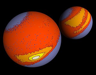
In directional statistics, the Kent distribution, also known as the 5-parameter Fisher–Bingham distribution, is a probability distribution on the unit sphere. It is the analogue on S2 of the bivariate normal distribution with an unconstrained covariance matrix. The Kent distribution was proposed by John T. Kent in 1982, and is used in geology as well as bioinformatics.

Bayesian linear regression is a type of conditional modeling in which the mean of one variable is described by a linear combination of other variables, with the goal of obtaining the posterior probability of the regression coefficients and ultimately allowing the out-of-sample prediction of the regressandconditional on observed values of the regressors. The simplest and most widely used version of this model is the normal linear model, in which given is distributed Gaussian. In this model, and under a particular choice of prior probabilities for the parameters—so-called conjugate priors—the posterior can be found analytically. With more arbitrarily chosen priors, the posteriors generally have to be approximated.

In statistics, the multivariate t-distribution is a multivariate probability distribution. It is a generalization to random vectors of the Student's t-distribution, which is a distribution applicable to univariate random variables. While the case of a random matrix could be treated within this structure, the matrix t-distribution is distinct and makes particular use of the matrix structure.

In quantum mechanics, the Pauli equation or Schrödinger–Pauli equation is the formulation of the Schrödinger equation for spin-1/2 particles, which takes into account the interaction of the particle's spin with an external electromagnetic field. It is the non-relativistic limit of the Dirac equation and can be used where particles are moving at speeds much less than the speed of light, so that relativistic effects can be neglected. It was formulated by Wolfgang Pauli in 1927. In its linearized form it is known as Lévy-Leblond equation.

In fluid dynamics and electrostatics, slender-body theory is a methodology that can be used to take advantage of the slenderness of a body to obtain an approximation to a field surrounding it and/or the net effect of the field on the body. Principal applications are to Stokes flow — at very low Reynolds numbers — and in electrostatics.

In probability theory and statistics, the negative multinomial distribution is a generalization of the negative binomial distribution (NB(x0, p)) to more than two outcomes.

<span class="mw-page-title-main">Bivariate von Mises distribution</span> Probability distribution on a torus

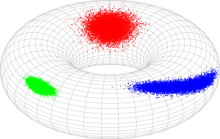
In probability theory and statistics, the bivariate von Mises distribution is a probability distribution describing values on a torus. It may be thought of as an analogue on the torus of the bivariate normal distribution. The distribution belongs to the field of directional statistics. The general bivariate von Mises distribution was first proposed by Kanti Mardia in 1975. One of its variants is today used in the field of bioinformatics to formulate a probabilistic model of protein structure in atomic detail, such as backbone-dependent rotamer libraries.

<span class="mw-page-title-main">Logit-normal distribution</span> Probability distribution

In probability theory, a logit-normal distribution is a probability distribution of a random variable whose logit has a normal distribution. If Y is a random variable with a normal distribution, and t is the standard logistic function, then X = t(Y) has a logit-normal distribution; likewise, if X is logit-normally distributed, then Y = logit(X)= log (X/(1-X)) is normally distributed. It is also known as the logistic normal distribution, which often refers to a multinomial logit version (e.g.).

The optical metric was defined by German theoretical physicist Walter Gordon in 1923 to study the geometrical optics in curved space-time filled with moving dielectric materials.

In the mathematical theory of probability, multivariate Laplace distributions are extensions of the Laplace distribution and the asymmetric Laplace distribution to multiple variables. The marginal distributions of symmetric multivariate Laplace distribution variables are Laplace distributions. The marginal distributions of asymmetric multivariate Laplace distribution variables are asymmetric Laplace distributions.

References

  1. Fisher, R. A. (1953). "Dispersion on a sphere". Proc. R. Soc. Lond. A. 217 (1130): 295–305. Bibcode:1953RSPSA.217..295F. doi:10.1098/rspa.1953.0064. S2CID   123166853.
  2. Watson, G. S. (1980). "Distributions on the Circle and on the Sphere". J. Appl. Probab. 19: 265–280. doi:10.2307/3213566. JSTOR   3213566. S2CID   222325569.
  3. 1 2 3 4 Mardia, Kanti; Jupp, P. E. (1999). Directional Statistics. John Wiley & Sons Ltd. ISBN   978-0-471-95333-3.
  4. Embleton, N. I. Fisher, T. Lewis, B. J. J. (1993). Statistical analysis of spherical data (1st pbk. ed.). Cambridge: Cambridge University Press. pp.  115–116. ISBN   0-521-45699-1.{{cite book}}: CS1 maint: multiple names: authors list (link)
  5. 1 2 Ulrich, Gary (1984). "Computer generation of distributions on the m-sphere". Applied Statistics. 33 (2): 158–163. doi:10.2307/2347441. JSTOR   2347441.
  6. Wood, Andrew T (1994). "Simulation of the Von Mises Fisher distribution". Communications in Statistics - Simulation and Computation. 23 (1): 157–164. doi:10.1080/03610919408813161.
  7. Hornik, Kurt; Grün, Bettina (2014). "movMF: An R Package for Fitting Mixtures of Von Mises-Fisher Distributions". Journal of Statistical Software. 58 (10). doi: 10.18637/jss.v058.i10 . S2CID   13171102.
  8. 1 2 Pinzón, Carlos; Jung, Kangsoo (2023-03-03), Fast Python sampler for the von Mises Fisher distribution , retrieved 2023-03-30
  9. De Cao, Nicola; Aziz, Wilker (13 Feb 2023). "The Power Spherical distribution". arXiv: 2006.04437 [stat.ML].
  10. Pakyuz-Charrier, Evren; Lindsay, Mark; Ogarko, Vitaliy; Giraud, Jeremie; Jessell, Mark (2018-04-06). "Monte Carlo simulation for uncertainty estimation on structural data in implicit 3-D geological modeling, a guide for disturbance distribution selection and parameterization". Solid Earth. 9 (2): 385–402. Bibcode:2018SolE....9..385P. doi: 10.5194/se-9-385-2018 . ISSN   1869-9510.
  11. A., Wood, Andrew T. (1992). Simulation of the Von Mises Fisher distribution. Centre for Mathematics & its Applications, Australian National University. OCLC   221030477.{{cite book}}: CS1 maint: multiple names: authors list (link)
  12. Gosmann, J; Eliasmith, C (2016). "Optimizing Semantic Pointer Representations for Symbol-Like Processing in Spiking Neural Networks". PLOS ONE. 11 (2): e0149928. Bibcode:2016PLoSO..1149928G. doi: 10.1371/journal.pone.0149928 . PMC   4762696 . PMID   26900931.
  13. 1 2 Voelker, Aaron R.; Gosmann, Jan; Stewart, Terrence C. "Efficiently sampling vectors and coordinates from the n-sphere and n-ball" (PDF). Centre for Theoretical Neuroscience – Technical Report, 2017. Retrieved 22 April 2023.
  14. Wang, Tongzhou; Isola, Phillip (2020). "Understanding Contrastive Representation Learning through Alignment and Uniformity on the Hypersphere". International Conference on Machine Learning (ICML). arXiv: 2005.10242 .
  15. Pal, Subhadip; Sengupta, Subhajit; Mitra, Riten; Banerjee, Arunava (2020). "Conjugate Priors and Posterior Inference for the Matrix Langevin Distribution on the Stiefel Manifold". Bayesian Analysis. 15 (3): 871–908. doi: 10.1214/19-BA1176 . ISSN   1936-0975.
  16. Chikuse, Yasuko (1 May 2003). "Concentrated matrix Langevin distributions". Journal of Multivariate Analysis. 85 (2): 375–394. doi: 10.1016/S0047-259X(02)00065-9 . ISSN   0047-259X.
  17. Jupp (1979). "Maximum likelihood estimators for the matrix von Mises-Fisher and Bingham distributions". The Annals of Statistics. 7 (3): 599–606. doi: 10.1214/aos/1176344681 .
  18. Downs (1972). "Orientational statistics". Biometrika. 59 (3): 665–676. doi:10.1093/biomet/59.3.665.
  19. Saw, John G (1978). "A family of distributions on the m-sphere and some hypothesis tests". Biometrika. 65 (`): 69–73. doi:10.2307/2335278. JSTOR   2335278.

Further reading