Charge based boundary element fast multipole method

The charge-based formulation of the boundary element method (BEM) is a dimensionality reduction numerical technique that is used to model quasistatic electromagnetic phenomena in highly complex conducting media (targeting, e.g., the human brain) with a very large (up to approximately 1 billion) number of unknowns. The charge-based BEM solves an integral equation of the potential theory ^[1] written in terms of the induced surface charge density. This formulation is naturally combined with fast multipole method (FMM) acceleration, and the entire method is known as charge-based BEM-FMM. The combination of BEM and FMM is a common technique in different areas of computational electromagnetics and, in the context of bioelectromagnetism, it provides improvements over the finite element method. ^{[2] [3] [4]}

Historical development

Along with more common electric potential-based BEM, ^{[5] [6]} the quasistatic charge-based BEM, derived in terms of the single-layer (charge) density, for a single-compartment medium has been known in the potential theory ^[1] since the beginning of the 20th century. For multi-compartment conducting media, the surface charge density formulation first appeared in discretized form (for faceted interfaces) in the 1964 paper by Gelernter and Swihart. ^[7] A subsequent continuous form, including time-dependent and dielectric effects, appeared in the 1967 paper by Barnard, Duck, and Lynn. ^[8] The charge-based BEM has also been formulated for conducting, dielectric, and magnetic media, ^[9] and used in different applications. ^[10]

In 2009, Greengard et al. ^[11] successfully applied the charge-based BEM with fast multipole acceleration to molecular electrostatics of dielectrics. A similar approach to realistic modeling of the human brain with multiple conducting compartments was first described by Makarov et al. ^[12] in 2018. Along with this, the BEM-based multilevel fast multipole method has been widely used in radar and antenna studies at microwave frequencies ^[13] as well as in acoustics. ^{[14] [15]}

Physical background - surface charges in biological media

The charge-based BEM is based on the concept of an impressed (or primary) electric field ${\displaystyle \mathbf {E} ^{i}}$ and a secondary electric field ${\displaystyle \mathbf {E} ^{s}}$. The impressed field is usually known a priori or is trivial to find. For the human brain, the impressed electric field can be classified as one of the following:

1. A conservative field ${\displaystyle \mathbf {E} ^{i}}$ derived from an impressed density of EEG or MEG current sources in a homogeneous infinite medium with the conductivity ${\displaystyle \sigma }$ at the source location; ^[16]
2. An instantaneous solenoidal field ${\displaystyle \mathbf {E} ^{i}}$ of an induction coil obtained from Faraday's law of induction in a homogeneous infinite medium (air), when transcranial magnetic stimulation (TMS) problems are concerned; ^{[12] [17]}
3. A surface field ${\displaystyle \mathbf {E} ^{i}}$derived from an impressed surface current density ${\displaystyle \mathbf {J} ^{i}=\sigma \mathbf {E} ^{i}}$ of current electrodes injecting electric current at a boundary of a compartment with conductivity ${\displaystyle \sigma }$ when transcranial direct-current stimulation (tDCS) or deep brain stimulation (DBS) are concerned; ^[18]
4. A conservative field ${\displaystyle \mathbf {E} ^{i}}$ of charges deposited on voltage electrodes for tDCS or DBS. This specific problem requires a coupled treatment since these charges will depend on the environment; ^[18]
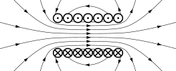
5. In application to multiscale modeling, a field ${\displaystyle \mathbf {E} ^{i}}$ obtained from any other macroscopic numerical solution in a small (mesoscale or microscale) spatial domain within the brain. For example, a constant field can be used. ^[19]

   

   Examples of impressed electric field for brain stimulation (TMS/DBS/tDCS/ICMS) and neurophysiological recordings (EEG/MEG). WM is white matter, GM - grey matter, and CSF - cerebrospinal fluid.

When the impressed field is "turned on", free charges located within a conducting volume D immediately begin to redistribute and accumulate at the boundaries (interfaces) of regions of different conductivity in D. A surface charge density ${\displaystyle \rho (\mathbf {r} )}$ appears on the conductivity interfaces. This charge density induces a secondary conservative electric field ${\displaystyle \mathbf {E} ^{s}}$ following Coulomb's law.

One example is a human under a direct current powerline with the known field ${\displaystyle \mathbf {E} ^{i}}$ directed down. The superior surface of the human's conducting body will be charged negatively while its inferior portion is charged positively. These surface charges create a secondary electric field that effectively cancels or blocks the primary field everywhere in the body so that no current will flow within the body under DC steady state conditions.

Another example is a human head with electrodes attached. At any conductivity interface with a normal vector ${\displaystyle \mathbf {n} }$ pointing from an "inside" (-) compartment of conductivity ${\displaystyle \sigma ^{-}}$to an "outside" (+) compartment of conductivity ${\displaystyle \sigma ^{+}}$, Kirchhoff's current law requires continuity of the normal component of the electric current density. This leads to the interfacial boundary condition in the form

${\displaystyle \sigma ^{+}\mathbf {E} ^{+}\cdot \mathbf {n} =\sigma ^{-}\mathbf {E} ^{-}\cdot \mathbf {n} }$

for every facet at a triangulated interface. As long as ${\displaystyle \sigma ^{\pm }}$ are different from each other, the two normal components of the electric field, ${\displaystyle \mathbf {E} ^{\pm }\cdot \mathbf {n} }$, must also be different. Such a jump across the interface is only possible when a sheet of surface charge exists at that interface. Thus, if an electric current or voltage is applied, the surface charge density follows.

The goal of the numerical analysis is to find the unknown surface charge distribution and thus the total electric field ${\displaystyle \mathbf {E} =\mathbf {E} ^{i}+\mathbf {E} ^{s}}$ (and the total electric potential if required) anywhere in space.

Derivation of discrete BEM-FMM using Gauss's law and Coulomb's law. Gauss's law applied to a "pillbox" located on the m-th facet can be used (in combination with Coulomb's law applied to all other facets) to give an approximation of the electric field just inside and outside every facet.

System of equations for surface charges

Below, a derivation is given based on Gauss's law and Coulomb's law. All conductivity interfaces, denoted by S, are discretized into planar triangular facets ${\displaystyle t_{m}}$ with centers ${\displaystyle \mathbf {r} _{m}}$. Assume that an m-th facet with the normal vector ${\displaystyle \mathbf {n} _{m}}$ and area ${\displaystyle A_{m}}$ carries a uniform surface charge density ${\displaystyle \rho _{m}}$. If a volumetric tetrahedral mesh were present, the charged facets would belong to tetrahedra with different conductivity values. We first compute the electric field ${\displaystyle \mathbf {E} _{m}^{+}}$ at the point ${\displaystyle \mathbf {r} _{m}+\delta \mathbf {n} _{m}}$, for ${\displaystyle \delta \rightarrow 0^{+}}$ i.e., just outside facet 𝑚 at its center. This field contains three contributions:

• The continuous impressed electric field ${\displaystyle \mathbf {E} ^{i}}$ itself;
• An electric field of the m-th charged facet itself. Very close to the facet, it can be approximated as the electric field of an infinite sheet of uniform surface charge ${\displaystyle \rho _{m}}$. ^[20] By Gauss's Law, it is given by ${\displaystyle +\rho _{m}/2\varepsilon _{0}\cdot \mathbf {n} _{m}}$ where ${\displaystyle \varepsilon _{0}}$ is a background electrical permittivity;
• An electric field generated by all other facets ${\displaystyle t_{n}}$, which we approximate as point charges of charge ${\displaystyle A_{n}\rho _{n}}$ at each center ${\displaystyle \mathbf {r} _{n}}$.

A similar treatment holds for the electric field ${\displaystyle \mathbf {E} _{m}^{-}}$ just inside facet 𝑚, but the electric field of the flat sheet of charge changes its sign. Using Coulomb's law to calculate the contribution of facets different from ${\displaystyle t_{m}}$, we find

${\displaystyle \mathbf {E} _{m}^{\pm }=\pm {\frac {\rho _{m}}{2\varepsilon _{0}}}\mathbf {n} _{m}+\sum _{n=1;n\neq m}^{M}{\frac {\rho _{n}}{4\pi \varepsilon _{0}}}{\frac {\mathbf {r} _{m}-\mathbf {r} _{n}}{|\mathbf {r} _{m}-\mathbf {r} _{n}|^{3}}}+\mathbf {E} ^{i}(\mathbf {r} _{m}),\ m=1,2,\dots ,M}$

From this equation, we see that the normal component of the electric field indeed undergoes a jump through the charged interface. This is equivalent to a jump relation of the potential theory. ^[1] As a second step, the two expressions for ${\displaystyle \mathbf {E} _{m}^{\pm }}$ are substituted into the interfacial boundary condition ${\displaystyle \sigma ^{-}\mathbf {E} _{m}^{-}\cdot \mathbf {n} _{m}=\sigma ^{+}\mathbf {E} _{m}^{+}\cdot \mathbf {n} _{m}}$, applied to every facet 𝑚. This operation leads to a system of linear equations for unknown charge densities ${\displaystyle \rho _{m}}$ which solves the problem:

${\displaystyle \rho _{m}=K_{m}\mathbf {n} _{m}\cdot \underbrace {\sum _{n=1;n\neq m}^{M}{\frac {\rho _{n}}{2\pi }}{\frac {\mathbf {r} _{m}-\mathbf {r} _{n}}{|\mathbf {r} _{m}-\mathbf {r} _{n}|^{3}}}} +{2}\varepsilon _{0}K_{m}\mathbf {n} _{m}\cdot \mathbf {E} ^{i}(\mathbf {r} _{m}),\ m=1,2,\dots ,M}$

where ${\displaystyle K_{m}={\frac {\sigma ^{-}-\sigma ^{+}}{\sigma ^{-}+\sigma ^{+}}}}$ is the electric conductivity contrast at the m-th facet. The normalization constant ${\displaystyle \varepsilon _{0}}$ will cancel out after the solution is substituted in the expression for ${\displaystyle \mathbf {E} ^{s}}$ and becomes redundant.

Application of fast multipole method

For modern characterizations of brain topologies with ever-increasing levels of complexity, the above system of equations for ${\displaystyle \rho _{m}}$ is very large; it is therefore solved iteratively. An initial guess for ${\displaystyle \rho _{m}}$ is the last term on its right-hand side while the sum is ignored. Next, the sum is computed and the initial guess is refined, etc. This solution ^{[12] [21]} employs the simple Jacobi iterative method. The more rigorous generalized minimum residual method (GMRES) yields a much faster convergence of the BEM-FMM. ^{[2] [3] [16] [17] [18]} In either case, the major work is in computing the underbraced sum in the system of equations above for every ${\displaystyle {m}}$ at every iteration; this operation corresponds to a repetitive matrix-vector multiplication. However, one can recognize this sum as an electric field (times ${\displaystyle {\frac {1}{2\pi \epsilon _{0}}}}$) of ${\displaystyle {M}}$ charges to be computed at ${\displaystyle {M}}$ observation points. Such a computation is exactly the task of the fast multipole method, which performs fast matrix-by-vector multiplication in ${\displaystyle O(M\log {M})}$ or even ${\displaystyle O(M)}$ operations instead of ${\displaystyle O(M^{2})}$. The FMM3D library ^[22] realized in both Python and MATLAB can be used for this purpose. It is therefore unnecessary to form or store the dense system matrix typical for the standard BEM.

Continuous charge-based BEM. Near-field correction

The system of equations formulated above is derived with the collocation method and is less accurate. ^[11] The corresponding integral equation is obtained from the local jump relations of the potential theory ^[23] and the local interfacial boundary condition of normal electric current continuity. It is a Fredholm integral equation of the second kind

${\displaystyle \rho (\mathbf {r} )=K(\mathbf {r} )\mathbf {n} (\mathbf {r} )\cdot \int _{S}{\frac {\rho (\mathbf {r^{\prime }} )}{2\pi }}{\frac {\mathbf {r} -\mathbf {r^{\prime }} }{|\mathbf {r} -\mathbf {r^{\prime }} |^{3}}}ds(\mathbf {r^{\prime }} )+2\varepsilon _{0}K(\mathbf {r} )\mathbf {E} ^{i}(\mathbf {r} )\cdot \mathbf {n} (\mathbf {r} ),\mathbf {r} {\text{ on }}S}$

Its derivation does not involve Green's identities (integrations by parts) and is applicable to non-nested geometries. When the Galerkin method is applied and the same zeroth-order basis functions (with a constant charge density for each facet) are still used on triangulated interfaces, we obtain exactly the same discretization as before if we replace the double integrals over surfaces ${\displaystyle S_{m}}$ and ${\displaystyle S_{n}}$ of triangles ${\displaystyle t_{m}}$ and ${\displaystyle t_{n}}$, respectively, by

${\displaystyle \int _{S_{m}}\int _{S_{n}}{\frac {\mathbf {r} -\mathbf {r^{\prime }} }{|\mathbf {r} -\mathbf {r^{\prime }} |^{3}}}ds(\mathbf {r^{\prime }} )ds(\mathbf {r} )\approx {A_{m}}{A_{n}}{\frac {\mathbf {r} _{m}-\mathbf {r} _{n}}{|\mathbf {r} _{m}-\mathbf {r} _{n}|^{3}}},}$

where ${\displaystyle {A_{n}}}$ is the surface area of the triangle ${\displaystyle {t_{n}}}$. This approximation is only valid when ${\displaystyle |\mathbf {r} _{m}-\mathbf {r} _{n}|}$ is much larger than a typical facet size i.e., in the "far field". Otherwise, semi-analytical formulae ^{[24] [25]} and Gaussian quadratures for triangles ^[26] should be used ^[12] . Typically, 4 to 32 such neighbor integrals per facet should be precomputed, stored, and then used at every iteration. ^{[12] [2] [17] [18] [27]} This is an important correction to the plain fast multipole method in the "near field" which should also be used in the simple discrete formulation derived above. Such a correction makes it possible to obtain an unconstrained numerical (but not anatomical) resolution in the brain. ^[17]

Applications and limitations

Applications of the charge-based BEM-FMM include modeling brain stimulation ^{[3] [17] [18] [21]} with near real-time accurate TMS computations ^{[28] [4]} as well as neurophysiological recordings. ^[16] They also include modeling challenging mesoscale head topologies such as thin brain membranes ^{[29] [27]} (dura mater, arachnoid mater, and pia mater). This is particularly important for accurate transcranial direct-current stimulation and electroconvulsive therapy dosage predictions. ^[30] The BEM-FMM allows for straightforward adaptive mesh refinement including multiple extracerebral brain compartments. ^{[27] [29]} Another application is modeling electric field perturbations within densely packed neuronal/axonal arbor. ^[19] Such perturbations change the biophysical activating function. A charge-based BEM formulation is being developed for promising bi-domain biophysical modeling of axonal processes. ^[31]

In its present form, the charge-based BEM-FMM is applicable to multi-compartment piecewise homogeneous media only; it cannot handle macroscopically anisotropic tissues. Additionally, the maximum number of facets (degrees of freedom) is limited to approximately ${\displaystyle 10^{9}}$ for typical academic computer hardware resources used as of 2023.

See also

• Computational electromagnetics
• Boundary element method
• Fast multipole method
• Computational neuroscience
• Transcranial magnetic stimulation
• Transcranial direct-current stimulation
• Electroencephalography
• Magnetoencephalography

External links

• A survey on integral equations for bioelectric modeling, preprint.
• Flatiron Institute - Simons Foundation FMM3D GitHub Project Site.

References

1. Kress, Rainer (1999). Linear Integral Equations (2 ed.). Springer. ISBN   9780387987002.
2. Htet, Aung Thu; Saturnino, Guilherme B; Burnham, Edward H; Noetscher, Gregory M; Nummenmaa, Aapo; Makarov, Sergey N (2019-04-01). "Comparative performance of the finite element method and the boundary element fast multipole method for problems mimicking transcranial magnetic stimulation (TMS)". Journal of Neural Engineering. 16 (2): 024001. doi:10.1088/1741-2552/aafbb9. ISSN   1741-2560. PMC   6546501 . PMID   30605893.
3. Gomez, Luis J.; Dannhauer, Moritz; Koponen, Lari M.; Peterchev, Angel V. (January 2020). "Conditions for numerically accurate TMS electric field simulation". Brain Stimulation. 13 (1): 157–166. doi:10.1016/j.brs.2019.09.015. PMC   6888902 . PMID   31604625.
4. Makaroff, S. N.; Qi, Z.; Rachh, M.; Wartman, W. A.; Weise, K.; Noetscher, G. M.; Daneshzand, M.; Deng, Zhi-De; Greengard, L.; Nummenmaa, A. R. (2023-10-31). "A fast direct solver for surface-based whole-head modeling of transcranial magnetic stimulation". Scientific Reports. 13 (1): 18657. Bibcode:2023NatSR..1318657M. doi:10.1038/s41598-023-45602-5. ISSN   2045-2322. PMC   10618282 . PMID   37907689.
5. Sarvas, J. (January 1987). "Basic mathematical and electromagnetic concepts of the biomagnetic inverse problem". Physics in Medicine and Biology. 32 (1): 11–22. Bibcode:1987PMB....32...11S. doi:10.1088/0031-9155/32/1/004. ISSN   0031-9155. PMID   3823129. S2CID   250776806.
6. Mosher, J. C.; Leahy, R. M.; Lewis, P. S. (March 1999). "EEG and MEG: forward solutions for inverse methods". IEEE Transactions on Biomedical Engineering. 46 (3): 245–259. doi:10.1109/10.748978. ISSN   0018-9294. PMID   10097460. S2CID   5323152.
7. Gelernter, H. L.; Swihart, J. C. (July 1964). "A Mathematical-Physical Model of the Genesis of the Electrocardiogram". Biophysical Journal. 4 (4): 285–301. Bibcode:1964BpJ.....4..285G. doi:10.1016/s0006-3495(64)86783-7. ISSN   0006-3495. PMC   1367507 . PMID   14197788.
8. Barnard, A. C.; Duck, I. M.; Lynn, M. S. (September 1967). "The application of electromagnetic theory to electrocardiology. I. Derivation of the integral equations". Biophysical Journal. 7 (5): 443–462. Bibcode:1967BpJ.....7..443B. doi:10.1016/S0006-3495(67)86598-6. ISSN   0006-3495. PMC   1368073 . PMID   6048873.
9. Makarov, Sergey N.; Noetscher, Gregory M.; Nazarian, Ara (2016). Low-frequency electromagnetic modeling for electrical and biological systems using MATLAB. Hoboken, New Jersey: Wiley. ISBN   978-1-119-05256-2.
10. Müller, E.; Petković, B.; Ziolkowski, M. (March 2024). "An Improved GPU-Optimized Fictitious Surface Charge Method for Transcranial Magnetic Stimulation". IEEE Trans. Magn. 60 (3): 1–4. Bibcode:2024ITM....6034747M. doi:10.1109/TMAG.2023.3334747.
11. Greengard, Leslie; Gueyffier, Denis; Martinsson, Per-Gunnar; Rokhlin, Vladimir (May 2009). "Fast direct solvers for integral equations in complex three-dimensional domains". Acta Numerica. 18: 243–275. doi:10.1017/S0962492906410011. ISSN   1474-0508. S2CID   58895952.
12. Makarov, Sergey N.; Noetscher, Gregory M.; Raij, Tommi; Nummenmaa, Aapo (December 2018). "A Quasi-Static Boundary Element Approach With Fast Multipole Acceleration for High-Resolution Bioelectromagnetic Models". IEEE Transactions on Biomedical Engineering. 65 (12): 2675–2683. doi:10.1109/TBME.2018.2813261. ISSN   0018-9294. PMC   7388683 . PMID   29993385.
13. Song, J.; Cai-Cheng Lu; Weng Cho Chew (October 1997). "Multilevel fast multipole algorithm for electromagnetic scattering by large complex objects". IEEE Transactions on Antennas and Propagation. 45 (10): 1488–1493. Bibcode:1997ITAP...45.1488S. doi:10.1109/8.633855.
14. Piscoya, Rafael; Ochmann, Martin (2015-03-01). "Acoustical Boundary Elements: Theory and Virtual Experiments". Archives of Acoustics. 39 (4): 453–465. doi:10.2478/aoa-2014-0049. ISSN   2300-262X. See also https://projekt.bht-berlin.de/ca/veroeffentlichungen/computational-acoustics-i-ii
15. Liu, Yijun (2009). Fast Multipole Boundary Element Method: Theory and Applications in Engineering. Cambridge: Cambridge University Press. doi:10.1017/cbo9780511605345. ISBN   978-0-521-11659-6.
16. Makarov, Sergey N.; Hamalainen, Matti; Okada, Yoshio; Noetscher, Gregory M.; Ahveninen, Jyrki; Nummenmaa, Aapo (January 2021). "Boundary Element Fast Multipole Method for Enhanced Modeling of Neurophysiological Recordings". IEEE Transactions on Biomedical Engineering. 68 (1): 308–318. doi:10.1109/TBME.2020.2999271. ISSN   0018-9294. PMC   7704617 . PMID   32746015.
17. Makarov, Sergey N; Wartman, William A; Daneshzand, Mohammad; Fujimoto, Kyoko; Raij, Tommi; Nummenmaa, Aapo (2020-08-04). "A software toolkit for TMS electric-field modeling with boundary element fast multipole method: an efficient MATLAB implementation". Journal of Neural Engineering. 17 (4): 046023. Bibcode:2020JNEng..17d6023M. doi:10.1088/1741-2552/ab85b3. ISSN   1741-2552. PMID   32235065. S2CID   213777043.
18. Makarov, Sergey N; Golestanirad, Laleh; Wartman, William A; Nguyen, Bach Thanh; Noetscher, Gregory M; Ahveninen, Jyrki P; Fujimoto, Kyoko; Weise, Konstantin; Nummenmaa, Aapo R (2021-08-01). "Boundary element fast multipole method for modeling electrical brain stimulation with voltage and current electrodes". Journal of Neural Engineering. 18 (4): 0460d4. Bibcode:2021JNEng..18d60d4M. doi:10.1088/1741-2552/ac17d7. ISSN   1741-2560. PMC   8783394 . PMID   34311449.
19. Noetscher, Gregory M.; Tang, Dexuan; Nummenmaa, Aapo R.; Bingham, Clayton S.; McIntyre, Cameron C.; Makaroff, Sergey N. (Jan 2024). "Estimations of Charge Deposition Onto Convoluted Axon Surfaces Within Extracellular Electric Fields". IEEE Transactions on Biomedical Engineering. 71 (1): 307–317. doi:10.1109/TBME.2023.3299734. ISSN   1558-2531. PMC   10837334 . PMID   37535481. S2CID   260487095.
20. "Electric Field, Flat Sheets of Charge". hyperphysics.phy-astr.gsu.edu. Retrieved 2023-12-29.
21. Müller, E.; Petković, B.; Ziolkowski, M.; Weise, K.; Toepfer, H.; Haueisen, J. (2023). "An Improved GPU Optimized Fictitious Surface Charge Method for Transcranial Magnetic Stimulation". IEEE Transactions on Magnetics. 60 (3): 1–4. Bibcode:2024ITM....6034747M. doi:10.1109/TMAG.2023.3334747. ISSN   0018-9464. S2CID   265559793.
22. Askham, Travis; Gimbutas, Zydrunas; Greengard, Leslie; Lu, Libin; Magland, Jeremy; Malhotra, Dhairya; O'Neil, Mike; Rachh, Manas; Rokhlin, Vladimir. "FMM3D Library". Flatiron Institute Fast Multipole Libraries. Flatiron Institute. Retrieved 15 December 2023.
23. Nuñez Ponasso G (2024). "A survey on integral equations for bioelectric modeling". Phys Med Biol. 69 (17): 17TR02. Bibcode:2024PMB....69T7R02P. doi:10.1088/1361-6560/ad66a9. PMC  11410390. PMID   39042098.
24. Zhongde Wang; Volakis, J.; Saitou, K.; Kurabayashi, K. (December 2003). "Comparison of semi-analytical formulations and gaussian-quadrature rules for quasi-static douwe-surface potential integrals". IEEE Antennas and Propagation Magazine. 45 (6): 96–102. Bibcode:2003IAPM...45...96W. doi:10.1109/MAP.2003.1282185. hdl: 2027.42/87252 . ISSN   1045-9243.
25. Wilton, D.; Rao, S.; Glisson, A.; Schaubert, D.; Al-Bundak, O.; Butler, C. (March 1984). "Potential integrals for uniform and linear source distributions on polygonal and polyhedral domains". IEEE Transactions on Antennas and Propagation. 32 (3): 276–281. Bibcode:1984ITAP...32..276W. doi:10.1109/TAP.1984.1143304. ISSN   0096-1973.
26. Stroud, A. H. (1971-01-01). Approximate Calculation of Multiple Integrals. Prentice-Hall.
27. Wartman, William A.; Weise, Konstantin; Rachh, Manas; Morales, Leah; Deng, Zhi-De; Nummenmaa, Aapo; Makaroff, Sergey N. (2023-08-15), "An Adaptive H-Refinement Method for the Boundary Element Fast Multipole Method for Quasi-static Electromagnetic Modeling", BioRxiv: The Preprint Server for Biology, doi:10.1101/2023.08.11.552996, PMC   10461998 , PMID   37645957 , retrieved 2023-12-25
28. Daneshzand, Mohammad; Makarov, Sergey N.; de Lara, Lucia I. Navarro; Guerin, Bastien; McNab, Jennifer; Rosen, Bruce R.; Hämäläinen, Matti S.; Raij, Tommi; Nummenmaa, Aapo (2021-08-15). "Rapid computation of TMS-induced E-fields using a dipole-based magnetic stimulation profile approach". NeuroImage. 237: 118097. doi:10.1016/j.neuroimage.2021.118097. ISSN   1095-9572. PMC   8353625 . PMID   33940151.
29. Weise, Konstantin; Wartman, William A.; Knösche, Thomas R.; Nummenmaa, Aapo R.; Makarov, Sergey N. (2022). "The effect of meninges on the electric fields in TES and TMS. Numerical modeling with adaptive mesh refinement". Brain Stimulation. 15 (3): 654–663. doi: 10.1016/j.brs.2022.04.009 . ISSN   1876-4754. PMID   35447379.
30. Deng, Zhi-De; Argyelan, Miklos; Miller, Jeremy; Quinn, Davin K.; Lloyd, Megan; Jones, Thomas R.; Upston, Joel; Erhardt, Erik; McClintock, Shawn M.; Abbott, Christopher C. (March 2022). "Electroconvulsive therapy, electric field, neuroplasticity, and clinical outcomes". Molecular Psychiatry. 27 (3): 1676–1682. doi:10.1038/s41380-021-01380-y. ISSN   1476-5578. PMC   9095458 . PMID   34853404.
31. Czerwonky DM, Aberra AS, Gomez LJ (2024). "A boundary element method of bidomain modeling for predicting cellular responses to electromagnetic fields". J Neural Eng. 21 (3): 036050. Bibcode:2024JNEng..21c6050C. doi: 10.1088/1741-2552/ad5704 . PMID   38862011.