In economics, utility is a measure of the satisfaction that a certain person has from a certain state of the world. Over time, the term has been used in at least two different meanings.

In economics, an indifference curve connects points on a graph representing different quantities of two goods, points between which a consumer is indifferent. That is, any combinations of two products indicated by the curve will provide the consumer with equal levels of utility, and the consumer has no preference for one combination or bundle of goods over a different combination on the same curve. One can also refer to each point on the indifference curve as rendering the same level of utility (satisfaction) for the consumer. In other words, an indifference curve is the locus of various points showing different combinations of two goods providing equal utility to the consumer. Utility is then a device to represent preferences rather than something from which preferences come. The main use of indifference curves is in the representation of potentially observable demand patterns for individual consumers over commodity bundles.
In economics, elasticity measures the responsiveness of one economic variable to a change in another. If the price elasticity of the demand of something is -2, a 10% increase in price causes the quantity demanded to fall by 20%. Elasticity in economics provides an understanding of changes in the behavior of the buyers and sellers with price changes. There are two types of elasticity for demand and supply, one is inelastic demand and supply and the other one is elastic demand and supply.
The theory of consumer choice is the branch of microeconomics that relates preferences to consumption expenditures and to consumer demand curves. It analyzes how consumers maximize the desirability of their consumption, by maximizing utility subject to a consumer budget constraint. Factors influencing consumers' evaluation of the utility of goods include: income level, cultural factors, product information and physio-psychological factors.
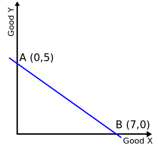
In economics, a budget constraint represents all the combinations of goods and services that a consumer may purchase given current prices within their given income. Consumer theory uses the concepts of a budget constraint and a preference map as tools to examine the parameters of consumer choices. Both concepts have a ready graphical representation in the two-good case. The consumer can only purchase as much as their income will allow, hence they are constrained by their budget. The equation of a budget constraint is where is the price of good X, and is the price of good Y, and m is income.

In economics, inferior goods are those goods the demand for which falls with increase in income of the consumer. So, there is an inverse relationship between income of the consumer and the demand for inferior goods. There are many examples of inferior goods, including cheap cars, public transit options, payday lending, and inexpensive food. The shift in consumer demand for an inferior good can be explained by two natural economic phenomena: the substitution effect and the income effect.

In microeconomics, substitute goods are two goods that can be used for the same purpose by consumers. That is, a consumer perceives both goods as similar or comparable, so that having more of one good causes the consumer to desire less of the other good. Contrary to complementary goods and independent goods, substitute goods may replace each other in use due to changing economic conditions. An example of substitute goods is Coca-Cola and Pepsi; the interchangeable aspect of these goods is due to the similarity of the purpose they serve, i.e. fulfilling customers' desire for a soft drink. These types of substitutes can be referred to as close substitutes.
In economics and particularly in consumer choice theory, the substitution effect is one component of the effect of a change in the price of a good upon the amount of that good demanded by a consumer, the other being the income effect.

In microeconomics, the law of demand is a fundamental principle which states that there is an inverse relationship between price and quantity demanded. In other words, "conditional on all else being equal, as the price of a good increases (↑), quantity demanded will decrease (↓); conversely, as the price of a good decreases (↓), quantity demanded will increase (↑)". Alfred Marshall worded this as: "When we say that a person's demand for anything increases, we mean that he will buy more of it than he would before at the same price, and that he will buy as much of it as before at a higher price". The law of demand, however, only makes a qualitative statement in the sense that it describes the direction of change in the amount of quantity demanded but not the magnitude of change.

In economics, a complementary good is a good whose appeal increases with the popularity of its complement. Technically, it displays a negative cross elasticity of demand and that demand for it increases when the price of another good decreases. If is a complement to , an increase in the price of will result in a negative movement along the demand curve of and cause the demand curve for to shift inward; less of each good will be demanded. Conversely, a decrease in the price of will result in a positive movement along the demand curve of and cause the demand curve of to shift outward; more of each good will be demanded. This is in contrast to a substitute good, whose demand decreases when its substitute's price decreases.
Utility maximization was first developed by utilitarian philosophers Jeremy Bentham and John Stuart Mill. In microeconomics, the utility maximization problem is the problem consumers face: "How should I spend my money in order to maximize my utility?" It is a type of optimal decision problem. It consists of choosing how much of each available good or service to consume, taking into account a constraint on total spending (income), the prices of the goods and their preferences.
In microeconomics, a consumer's Marshallian demand function is the quantity they demand of a particular good as a function of its price, their income, and the prices of other goods, a more technical exposition of the standard demand function. It is a solution to the utility maximization problem of how the consumer can maximize their utility for given income and prices. A synonymous term is uncompensated demand function, because when the price rises the consumer is not compensated with higher nominal income for the fall in their real income, unlike in the Hicksian demand function. Thus the change in quantity demanded is a combination of a substitution effect and a wealth effect. Although Marshallian demand is in the context of partial equilibrium theory, it is sometimes called Walrasian demand as used in general equilibrium theory.
In microeconomics, the Slutsky equation, named after Eugen Slutsky, relates changes in Marshallian (uncompensated) demand to changes in Hicksian (compensated) demand, which is known as such since it compensates to maintain a fixed level of utility.
In microeconomics, a consumer's Hicksian demand function or compensated demand function for a good is their quantity demanded as part of the solution to minimizing their expenditure on all goods while delivering a fixed level of utility. Essentially, a Hicksian demand function shows how an economic agent would react to the change in the price of a good, if the agent's income was compensated to guarantee the agent the same utility previous to the change in the price of the good—the agent will remain on the same indifference curve before and after the change in the price of the good. The function is named after John Hicks.
A relative price is the price of a commodity such as a good or service in terms of another; i.e., the ratio of two prices. A relative price may be expressed in terms of a ratio between the prices of any two goods or the ratio between the price of one good and the price of a market basket of goods.
A Lindahl tax is a form of taxation conceived by Erik Lindahl in which individuals pay for public goods according to their marginal benefits. In other words, they pay according to the amount of satisfaction or utility they derive from the consumption of an additional unit of the public good. Lindahl taxation is designed to maximize efficiency for each individual and provide the optimal level of a public good.

In microeconomics, the property of local nonsatiation (LNS) of consumer preferences states that for any bundle of goods there is always another bundle of goods arbitrarily close that is strictly preferred to it.

Independent goods are goods that have a zero cross elasticity of demand. Changes in the price of one good will have no effect on the demand for an independent good. Thus independent goods are neither complements nor substitutes.
In economics and consumer theory, quasilinear utility functions are linear in one argument, generally the numeraire. Quasilinear preferences can be represented by the utility function where is strictly concave. A useful property of the quasilinear utility function is that the Marshallian/Walrasian demand for does not depend on wealth and is thus not subject to a wealth effect; The absence of a wealth effect simplifies analysis and makes quasilinear utility functions a common choice for modelling. Furthermore, when utility is quasilinear, compensating variation (CV), equivalent variation (EV), and consumer surplus are algebraically equivalent. In mechanism design, quasilinear utility ensures that agents can compensate each other with side payments.
In economics, and in other social sciences, preference refers to an order by which an agent, while in search of an "optimal choice", ranks alternatives based on their respective utility. Preferences are evaluations that concern matters of value, in relation to practical reasoning. Individual preferences are determined by taste, need, ..., as opposed to price, availability or personal income. Classical economics assumes that people act in their best (rational) interest. In this context, rationality would dictate that, when given a choice, an individual will select an option that maximizes their self-interest. But preferences are not always transitive, both because real humans are far from always being rational and because in some situations preferences can form cycles, in which case there exists no well-defined optimal choice. An example of this is Efron dice.


