![]() | This article includes a list of references, related reading, or external links, but its sources remain unclear because it lacks inline citations .(July 2013) |
In mathematics – specifically, in stochastic analysis – an Itô diffusion is a solution to a specific type of stochastic differential equation. That equation is similar to the Langevin equation used in physics to describe the Brownian motion of a particle subjected to a potential in a viscous fluid. Itô diffusions are named after the Japanese mathematician Kiyosi Itô.
A (time-homogeneous) Itô diffusion in n-dimensional Euclidean space Rn is a process X : [0, +∞) × Ω → Rn defined on a probability space (Ω, Σ, P) and satisfying a stochastic differential equation of the form
where B is an m-dimensional Brownian motion and b : Rn → Rn and σ : Rn → Rn×m satisfy the usual Lipschitz continuity condition
for some constant C and all x, y ∈ Rn; this condition ensures the existence of a unique strong solution X to the stochastic differential equation given above. The vector field b is known as the drift coefficient of X; the matrix field σ is known as the diffusion coefficient of X. It is important to note that b and σ do not depend upon time; if they were to depend upon time, X would be referred to only as an Itô process , not a diffusion. Itô diffusions have a number of nice properties, which include
In particular, an Itô diffusion is a continuous, strongly Markovian process such that the domain of its characteristic operator includes all twice-continuously differentiable functions, so it is a diffusion in the sense defined by Dynkin (1965).
An Itô diffusion X is a sample continuous process, i.e., for almost all realisations Bt(ω) of the noise, Xt(ω) is a continuous function of the time parameter, t. More accurately, there is a "continuous version" of X, a continuous process Y so that
This follows from the standard existence and uniqueness theory for strong solutions of stochastic differential equations.
In addition to being (sample) continuous, an Itô diffusion X satisfies the stronger requirement to be a Feller-continuous process.
For a point x ∈ Rn, let Px denote the law of X given initial datum X0 = x, and let Ex denote expectation with respect to Px.
Let f : Rn → R be a Borel-measurable function that is bounded below and define, for fixed t ≥ 0, u : Rn → R by
The behaviour of the function u above when the time t is varied is addressed by the Kolmogorov backward equation, the Fokker–Planck equation, etc. (See below.)
An Itô diffusion X has the important property of being Markovian: the future behaviour of X, given what has happened up to some time t, is the same as if the process had been started at the position Xt at time 0. The precise mathematical formulation of this statement requires some additional notation:
Let Σ∗ denote the natural filtration of (Ω, Σ) generated by the Brownian motion B: for t ≥ 0,
It is easy to show that X is adapted to Σ∗ (i.e. each Xt is Σt-measurable), so the natural filtration F∗ = F∗X of (Ω, Σ) generated by X has Ft ⊆ Σt for each t ≥ 0.
Let f : Rn → R be a bounded, Borel-measurable function. Then, for all t and h ≥ 0, the conditional expectation conditioned on the σ-algebra Σt and the expectation of the process "restarted" from Xt satisfy the Markov property:
In fact, X is also a Markov process with respect to the filtration F∗, as the following shows:
The strong Markov property is a generalization of the Markov property above in which t is replaced by a suitable random time τ : Ω → [0, +∞] known as a stopping time. So, for example, rather than "restarting" the process X at time t = 1, one could "restart" whenever X first reaches some specified point p of Rn.
As before, let f : Rn → R be a bounded, Borel-measurable function. Let τ be a stopping time with respect to the filtration Σ∗ with τ < +∞ almost surely. Then, for all h ≥ 0,
Associated to each Itô diffusion, there is a second-order partial differential operator known as the generator of the diffusion. The generator is very useful in many applications and encodes a great deal of information about the process X. Formally, the infinitesimal generator of an Itô diffusion X is the operator A, which is defined to act on suitable functions f : Rn → R by
The set of all functions f for which this limit exists at a point x is denoted DA(x), while DA denotes the set of all f for which the limit exists for all x ∈ Rn. One can show that any compactly-supported C2 (twice differentiable with continuous second derivative) function f lies in DA and that
or, in terms of the gradient and scalar and Frobenius inner products,
The generator A for standard n-dimensional Brownian motion B, which satisfies the stochastic differential equation dXt = dBt, is given by
i.e., A = Δ/2, where Δ denotes the Laplace operator.
The generator is used in the formulation of Kolmogorov's backward equation. Intuitively, this equation tells us how the expected value of any suitably smooth statistic of X evolves in time: it must solve a certain partial differential equation in which time t and the initial position x are the independent variables. More precisely, if f ∈ C2(Rn; R) has compact support and u : [0, +∞) × Rn → R is defined by
then u(t, x) is differentiable with respect to t, u(t, ·) ∈ DA for all t, and u satisfies the following partial differential equation, known as Kolmogorov's backward equation:
The Fokker–Planck equation (also known as Kolmogorov's forward equation) is in some sense the "adjoint" to the backward equation, and tells us how the probability density functions of Xt evolve with time t. Let ρ(t, ·) be the density of Xt with respect to Lebesgue measure on Rn, i.e., for any Borel-measurable set S ⊆ Rn,
Let A∗ denote the Hermitian adjoint of A (with respect to the L2 inner product). Then, given that the initial position X0 has a prescribed density ρ0, ρ(t, x) is differentiable with respect to t, ρ(t, ·) ∈ DA* for all t, and ρ satisfies the following partial differential equation, known as the Fokker–Planck equation:
The Feynman–Kac formula is a useful generalization of Kolmogorov's backward equation. Again, f is in C2(Rn; R) and has compact support, and q : Rn → R is taken to be a continuous function that is bounded below. Define a function v : [0, +∞) × Rn → R by
The Feynman–Kac formula states that v satisfies the partial differential equation
Moreover, if w : [0, +∞) × Rn → R is C1 in time, C2 in space, bounded on K × Rn for all compact K, and satisfies the above partial differential equation, then w must be v as defined above.
Kolmogorov's backward equation is the special case of the Feynman–Kac formula in which q(x) = 0 for all x ∈ Rn.
The characteristic operator of an Itô diffusion X is a partial differential operator closely related to the generator, but somewhat more general. It is more suited to certain problems, for example in the solution of the Dirichlet problem.
The characteristic operator of an Itô diffusion X is defined by
where the sets U form a sequence of open sets Uk that decrease to the point x in the sense that
and
is the first exit time from U for X. denotes the set of all f for which this limit exists for all x ∈ Rn and all sequences {Uk}. If Ex[τU] = +∞ for all open sets U containing x, define
The characteristic operator and infinitesimal generator are very closely related, and even agree for a large class of functions. One can show that
and that
In particular, the generator and characteristic operator agree for all C2 functions f, in which case
Above, the generator (and hence characteristic operator) of Brownian motion on Rn was calculated to be ½Δ, where Δ denotes the Laplace operator. The characteristic operator is useful in defining Brownian motion on an m-dimensional Riemannian manifold (M, g): a Brownian motion onM is defined to be a diffusion on M whose characteristic operator in local coordinates xi, 1 ≤ i ≤ m, is given by ½ΔLB, where ΔLB is the Laplace-Beltrami operator given in local coordinates by
where [gij] = [gij]−1 in the sense of the inverse of a square matrix.
In general, the generator A of an Itô diffusion X is not a bounded operator. However, if a positive multiple of the identity operator I is subtracted from A then the resulting operator is invertible. The inverse of this operator can be expressed in terms of X itself using the resolvent operator.
For α > 0, the resolvent operatorRα, acting on bounded, continuous functions g : Rn → R, is defined by
It can be shown, using the Feller continuity of the diffusion X, that Rαg is itself a bounded, continuous function. Also, Rα and αI − A are mutually inverse operators:
Sometimes it is necessary to find an invariant measure for an Itô diffusion X, i.e. a measure on Rn that does not change under the "flow" of X: i.e., if X0 is distributed according to such an invariant measure μ∞, then Xt is also distributed according to μ∞ for any t ≥ 0. The Fokker–Planck equation offers a way to find such a measure, at least if it has a probability density function ρ∞: if X0 is indeed distributed according to an invariant measure μ∞ with density ρ∞, then the density ρ(t, ·) of Xt does not change with t, so ρ(t, ·) = ρ∞, and so ρ∞ must solve the (time-independent) partial differential equation
This illustrates one of the connections between stochastic analysis and the study of partial differential equations. Conversely, a given second-order linear partial differential equation of the form Λf = 0 may be hard to solve directly, but if Λ = A∗ for some Itô diffusion X, and an invariant measure for X is easy to compute, then that measure's density provides a solution to the partial differential equation.
An invariant measure is comparatively easy to compute when the process X is a stochastic gradient flow of the form
where β > 0 plays the role of an inverse temperature and Ψ : Rn → R is a scalar potential satisfying suitable smoothness and growth conditions. In this case, the Fokker–Planck equation has a unique stationary solution ρ∞ (i.e. X has a unique invariant measure μ∞ with density ρ∞) and it is given by the Gibbs distribution:
where the partition function Z is given by
Moreover, the density ρ∞ satisfies a variational principle: it minimizes over all probability densities ρ on Rn the free energy functional F given by
where
plays the role of an energy functional, and
is the negative of the Gibbs-Boltzmann entropy functional. Even when the potential Ψ is not well-behaved enough for the partition function Z and the Gibbs measure μ∞ to be defined, the free energy F[ρ(t, ·)] still makes sense for each time t ≥ 0, provided that the initial condition has F[ρ(0, ·)] < +∞. The free energy functional F is, in fact, a Lyapunov function for the Fokker–Planck equation: F[ρ(t, ·)] must decrease as t increases. Thus, F is an H-function for the X-dynamics.
Consider the Ornstein-Uhlenbeck process X on Rn satisfying the stochastic differential equation
where m ∈ Rn and β, κ > 0 are given constants. In this case, the potential Ψ is given by
and so the invariant measure for X is a Gaussian measure with density ρ∞ given by
Heuristically, for large t, Xt is approximately normally distributed with mean m and variance (βκ)−1. The expression for the variance may be interpreted as follows: large values of κ mean that the potential well Ψ has "very steep sides", so Xt is unlikely to move far from the minimum of Ψ at m; similarly, large values of β mean that the system is quite "cold" with little noise, so, again, Xt is unlikely to move far away from m.
In general, an Itô diffusion X is not a martingale. However, for any f ∈ C2(Rn; R) with compact support, the process M : [0, +∞) × Ω → R defined by
where A is the generator of X, is a martingale with respect to the natural filtration F∗ of (Ω, Σ) by X. The proof is quite simple: it follows from the usual expression of the action of the generator on smooth enough functions f and Itô's lemma (the stochastic chain rule) that
Since Itô integrals are martingales with respect to the natural filtration Σ∗ of (Ω, Σ) by B, for t > s,
Hence, as required,
since Ms is Fs-measurable.
Dynkin's formula, named after Eugene Dynkin, gives the expected value of any suitably smooth statistic of an Itô diffusion X (with generator A) at a stopping time. Precisely, if τ is a stopping time with Ex[τ] < +∞, and f : Rn → R is C2 with compact support, then
Dynkin's formula can be used to calculate many useful statistics of stopping times. For example, canonical Brownian motion on the real line starting at 0 exits the interval (−R, +R) at a random time τR with expected value
Dynkin's formula provides information about the behaviour of X at a fairly general stopping time. For more information on the distribution of X at a hitting time, one can study the harmonic measure of the process.
In many situations, it is sufficient to know when an Itô diffusion X will first leave a measurable set H ⊆ Rn. That is, one wishes to study the first exit time
Sometimes, however, one also wishes to know the distribution of the points at which X exits the set. For example, canonical Brownian motion B on the real line starting at 0 exits the interval (−1, 1) at −1 with probability ½ and at 1 with probability ½, so Bτ(−1, 1) is uniformly distributed on the set {−1, 1}.
In general, if G is compactly embedded within Rn, then the harmonic measure (or hitting distribution) of X on the boundary ∂G of G is the measure μGx defined by
for x ∈ G and F ⊆ ∂G.
Returning to the earlier example of Brownian motion, one can show that if B is a Brownian motion in Rn starting at x ∈ Rn and D ⊂ Rn is an open ball centred on x, then the harmonic measure of B on ∂D is invariant under all rotations of D about x and coincides with the normalized surface measure on ∂D.
The harmonic measure satisfies an interesting mean value property: if f : Rn → R is any bounded, Borel-measurable function and φ is given by
then, for all Borel sets G ⊂⊂ H and all x ∈ G,
The mean value property is very useful in the solution of partial differential equations using stochastic processes.
Let A be a partial differential operator on a domain D ⊆ Rn and let X be an Itô diffusion with A as its generator. Intuitively, the Green measure of a Borel set H is the expected length of time that X stays in H before it leaves the domain D. That is, the Green measure of X with respect to D at x, denoted G(x, ·), is defined for Borel sets H ⊆ Rn by
or for bounded, continuous functions f : D → R by
The name "Green measure" comes from the fact that if X is Brownian motion, then
where G(x, y) is Green's function for the operator ½Δ on the domain D.
Suppose that Ex[τD] < +∞ for all x ∈ D. Then the Green formula holds for all f ∈ C2(Rn; R) with compact support:
In particular, if the support of f is compactly embedded in D,
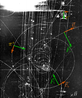
In physics, the Lorentz force is the combination of electric and magnetic force on a point charge due to electromagnetic fields. A particle of charge q moving with a velocity v in an electric field E and a magnetic field B experiences a force of
The Navier–Stokes equations are partial differential equations which describe the motion of viscous fluid substances, named after French engineer and physicist Claude-Louis Navier and Irish physicist and mathematician George Gabriel Stokes. They were developed over several decades of progressively building the theories, from 1822 (Navier) to 1842-1850 (Stokes).
In statistical mechanics and information theory, the Fokker–Planck equation is a partial differential equation that describes the time evolution of the probability density function of the velocity of a particle under the influence of drag forces and random forces, as in Brownian motion. The equation can be generalized to other observables as well. The Fokker-Planck equation has multiple applications in information theory, graph theory, data science, finance, economics etc.
In mathematics, the Laplace operator or Laplacian is a differential operator given by the divergence of the gradient of a scalar function on Euclidean space. It is usually denoted by the symbols , (where is the nabla operator), or . In a Cartesian coordinate system, the Laplacian is given by the sum of second partial derivatives of the function with respect to each independent variable. In other coordinate systems, such as cylindrical and spherical coordinates, the Laplacian also has a useful form. Informally, the Laplacian Δf (p) of a function f at a point p measures by how much the average value of f over small spheres or balls centered at p deviates from f (p).
In mathematics, Itô's lemma or Itô's formula is an identity used in Itô calculus to find the differential of a time-dependent function of a stochastic process. It serves as the stochastic calculus counterpart of the chain rule. It can be heuristically derived by forming the Taylor series expansion of the function up to its second derivatives and retaining terms up to first order in the time increment and second order in the Wiener process increment. The lemma is widely employed in mathematical finance, and its best known application is in the derivation of the Black–Scholes equation for option values.
Linear elasticity is a mathematical model of how solid objects deform and become internally stressed due to prescribed loading conditions. It is a simplification of the more general nonlinear theory of elasticity and a branch of continuum mechanics.
The Feynman–Kac formula, named after Richard Feynman and Mark Kac, establishes a link between parabolic partial differential equations (PDEs) and stochastic processes. In 1947, when Kac and Feynman were both Cornell faculty, Kac attended a presentation of Feynman's and remarked that the two of them were working on the same thing from different directions. The Feynman–Kac formula resulted, which proves rigorously the real case of Feynman's path integrals. The complex case, which occurs when a particle's spin is included, is still an open question.
In physics, the Hamilton–Jacobi equation, named after William Rowan Hamilton and Carl Gustav Jacob Jacobi, is an alternative formulation of classical mechanics, equivalent to other formulations such as Newton's laws of motion, Lagrangian mechanics and Hamiltonian mechanics.
In stochastic processes, the Stratonovich integral or Fisk–Stratonovich integral is a stochastic integral, the most common alternative to the Itô integral. Although the Itô integral is the usual choice in applied mathematics, the Stratonovich integral is frequently used in physics.
Toroidal coordinates are a three-dimensional orthogonal coordinate system that results from rotating the two-dimensional bipolar coordinate system about the axis that separates its two foci. Thus, the two foci and in bipolar coordinates become a ring of radius in the plane of the toroidal coordinate system; the -axis is the axis of rotation. The focal ring is also known as the reference circle.
In mathematics, parabolic cylindrical coordinates are a three-dimensional orthogonal coordinate system that results from projecting the two-dimensional parabolic coordinate system in the perpendicular -direction. Hence, the coordinate surfaces are confocal parabolic cylinders. Parabolic cylindrical coordinates have found many applications, e.g., the potential theory of edges.
The shallow-water equations (SWE) are a set of hyperbolic partial differential equations that describe the flow below a pressure surface in a fluid. The shallow-water equations in unidirectional form are also called Saint-Venant equations, after Adhémar Jean Claude Barré de Saint-Venant.
There are various mathematical descriptions of the electromagnetic field that are used in the study of electromagnetism, one of the four fundamental interactions of nature. In this article, several approaches are discussed, although the equations are in terms of electric and magnetic fields, potentials, and charges with currents, generally speaking.
The intent of this article is to highlight the important points of the derivation of the Navier–Stokes equations as well as its application and formulation for different families of fluids.
In mathematics — specifically, in stochastic analysis — Dynkin's formula is a theorem giving the expected value of any suitably smooth statistic of an Itō diffusion at a stopping time. It may be seen as a stochastic generalization of the (second) fundamental theorem of calculus. It is named after the Russian mathematician Eugene Dynkin.
In mathematics — specifically, in stochastic analysis — the Green measure is a measure associated to an Itō diffusion. There is an associated Green formula representing suitably smooth functions in terms of the Green measure and first exit times of the diffusion. The concepts are named after the British mathematician George Green and are generalizations of the classical Green's function and Green formula to the stochastic case using Dynkin's formula.
In the theory of stochastic processes, filtering describes the problem of determining the state of a system from an incomplete and potentially noisy set of observations. While originally motivated by problems in engineering, filtering found applications in many fields from signal processing to finance.
The Cauchy momentum equation is a vector partial differential equation put forth by Cauchy that describes the non-relativistic momentum transport in any continuum.
Lagrangian field theory is a formalism in classical field theory. It is the field-theoretic analogue of Lagrangian mechanics. Lagrangian mechanics is used to analyze the motion of a system of discrete particles each with a finite number of degrees of freedom. Lagrangian field theory applies to continua and fields, which have an infinite number of degrees of freedom.
Quantum stochastic calculus is a generalization of stochastic calculus to noncommuting variables. The tools provided by quantum stochastic calculus are of great use for modeling the random evolution of systems undergoing measurement, as in quantum trajectories. Just as the Lindblad master equation provides a quantum generalization to the Fokker–Planck equation, quantum stochastic calculus allows for the derivation of quantum stochastic differential equations (QSDE) that are analogous to classical Langevin equations.