This article is being considered for deletion in accordance with Wikipedia's deletion policy. Please share your thoughts on the matter at this article's deletion discussion page.
Feel free to improve the article, but do not remove this notice before the discussion is closed and do not blank the page. For more information, read the guide to deletion. Find sources:"Defining equation"physics–news·newspapers·books·scholar·JSTOR%5B%5BWikipedia%3AArticles+for+deletion%2FDefining+equation+%28physics%29%5D%5DAFD
Defining quantities is analogous to mixing colours, and could be classified a similar way, although this is not standard. Primary colours are to base quantities; as secondary (or tertiary etc.) colours are to derived quantities. Mixing colours is analogous to combining quantities using mathematical operations. But colours could be for light or paint, and analogously the system of units could be one of many forms: such as SI (now most common), CGS, Gaussian, old imperial units, a specific form of natural units or even arbitrarily defined units characteristic to the physical system in consideration (characteristic units).
The choice of a base system of quantities and units is arbitrary; but once chosen it must be adhered to throughout all analysis which follows for consistency. It makes no sense to mix up different systems of units. Choosing a system of units, one system out of the SI, CGS etc., is like choosing whether use paint or light colours.
In light of this analogy, primary definitions are base quantities with no defining equation, but defined standardized condition, "secondary" definitions are quantities defined purely in terms of base quantities, "tertiary" for quantities in terms of both base and "secondary" quantities, "quaternary" for quantities in terms of base, "secondary", and "tertiary" quantities, and so on.
Motivation
Much of physics requires definitions to be made for the equations to make sense.
Theoretical implications: Definitions are important since they can lead into new insights of a branch of physics. Two such examples occurred in classical physics. When entropyS was defined – the range of thermodynamics was greatly extended by associating chaos and disorder with a numerical quantity that could relate to energy and temperature, leading to the understanding of the secondthermodynamic law and statistical mechanics.[2]
Analytical convenience: They allow other equations to be written more compactly and so allow easier mathematical manipulation; by including a parameter in a definition, occurrences of the parameter can be absorbed into the substituted quantity and removed from the equation.[4]
which is simpler to write, even if the equation is the same.
Ease of comparison: They allow comparisons of measurements to be made when they might appear ambiguous and unclear otherwise.
Example
A basic example is mass density. It is not clear how compare how much matter constitutes a variety of substances given only their masses or only their volumes. Given both for each substance, the mass m per unit volume V, or mass density ρ provides a meaningful comparison between the substances, since for each, a fixed amount of volume will correspond to an amount of mass depending on the substance. To illustrate this; if two substances A and B have masses mA and mB respectively, occupying volumes VA and VB respectively, using the definition of mass density gives:
ρA = mA / VA , ρB = mB / VB
following this can be seen that:
if mA > mB or mA < mB and VA = VB, then ρA > ρB or ρA < ρB,
if mA = mB and VA > VB or VA < VB, then ρA < ρB or ρA > ρB,
if ρA = ρB, then mA / VA = mB / VB so mA / mB = VA / VB, demonstrating that if mA > mB or mA < mB, then VA > VB or VA < VB.
Making such comparisons without using mathematics logically in this way would not be as systematic.
Construction of defining equations
Scope of definitions
Defining equations are normally formulated in terms of elementary algebra and calculus, vector algebra and calculus, or for the most general applications tensor algebra and calculus, depending on the level of study and presentation, complexity of topic and scope of applicability. Functions may be incorporated into a definition, in for calculus this is necessary. Quantities may also be complex-valued for theoretical advantage, but for a physical measurement the real part is relevant, the imaginary part can be discarded. For more advanced treatments the equation may have to be written in an equivalent but alternative form using other defining equations for the definition to be useful. Often definitions can start from elementary algebra, then modify to vectors, then in the limiting cases calculus may be used. The various levels of maths used typically follows this pattern.
Typically definitions are explicit, meaning the defining quantity is the subject of the equation, but sometimes the equation is not written explicitly – although the defining quantity can be solved for to make the equation explicit. For vector equations, sometimes the defining quantity is in a cross or dot product and cannot be solved for explicitly as a vector, but the components can.
Electric current density is an example spanning all of these methods, Angular momentum is an example which doesn't require calculus. See the classical mechanics section below for nomenclature and diagrams to the right.
Elementary algebra
Operations are simply multiplication and division. Equations may be written in a product or quotient form, both of course equivalent.
Angular momentum
Electric current density
Quotient form
Product form
Vector algebra
There is no way to divide a vector by a vector, so there are no product or quotient forms.
Angular momentum
Electric current density
Quotient form
N/A
Product form
Starting from
since L = 0 when p and r are parallel or antiparallel, and is a maximum when perpendicular, so that the only component of p which contributes to L is the tangential |p| sin θ, the magnitude of angular momentum L should be re-written as
Since r, p and L form a right-hand triad, this leads to the vector form
Elementary calculus
The arithmetic operations are modified to the limiting cases of differentiation and integration. Equations can be expressed in these equivalent and alternative ways.
Sometimes there is still freedom within the chosen units system, to define one or more quantities in more than one way. The situation splits into two cases:[6]
Mutually exclusive definitions: There are a number of possible choices for a quantity to be defined in terms of others, but only one can be used and not the others. Choosing more than one of the exclusive equations for a definition leads to a contradiction – one equation might demand a quantity X to be defined in one way using another quantity Y, while another equation requires the reverse, Y be defined using X, but then another equation might falsify the use of both X and Y, and so on. The mutual disagreement makes it impossible to say which equation defines what quantity.
Equivalent definitions: Defining equations which are equivalent and self-consistent with other equations and laws within the physical theory, simply written in different ways.
There are two possibilities for each case:
One defining equation – one defined quantity: A defining equation is used to define a single quantity in terms of a number of others.
One defining equation – a number of defined quantities: A defining equation is used to define a number of quantities in terms of a number of others. A single defining equation shouldn't contain one quantity defining all other quantities in the same equation, otherwise contradictions arise again. There is no definition of the defined quantities separately since they are defined by a single quantity in a single equation. Furthermore, the defined quantities may have already been defined before, so if another quantity defines these in the same equation, there is a clash between definitions.
Contradictions can be avoided by defining quantities successively; the order in which quantities are defined must be accounted for. Examples spanning these instances occur in electromagnetism, and are given below.
where is the change in position traversed by the charge carriers (assuming current is independent of position, if not so a line integral must be done along the path of current) or in terms of the magnetic flux ΦB through a surface S, where the area is used as a scalar A and vector: and is a unit normal to A, either in differential form
or integral form,
However, only one of the above equations can be used to define B for the following reason, given that A, r, v, and F have been defined elsewhere unambiguously (most likely mechanics and Euclidean geometry).
If the force equation defines B, where q or I have been previously defined, then the flux equation defines ΦB, since B has been previously defined unambiguously. If the flux equation defines B, where ΦB, the force equation may be a defining equation for I or q. Notice the contradiction when B both equations define B simultaneously and when B is not a base quantity; the force equation demands that q or I be defined elsewhere while at the same time the flux equation demands that q or I be defined by the force equation, similarly the force equation requires ΦB to be defined by the flux equation, at the same time the flux equation demands that ΦB is defined elsewhere. For both equations to be used as definitions simultaneously, B must be a base quantity so that F and ΦB can be defined to stem from B unambiguously.[6]
Equivalent definitions:
Another example is inductanceL which has two equivalent equations to use as a definition.[7][8]
One defining equation – a number of defined quantities
Notice that L cannot define I and ΦB simultaneously - this makes no sense. I, ΦB and V have most likely all been defined before as (ΦB given above in flux equation);
where W = work done on charge q. Furthermore, there is no definition of either I or ΦB separately – because L is defining them in the same equation.
as a single defining equation for the electric fieldE and magnetic field B is allowed, since E and B are not only defined by one variable, but three; force F, velocity v and charge q. This is consistent with isolated definitions of E and B since E is defined using F and q:
and B defined by F, v, and q, as given above.
Limitations of definitions
Definitions vs. functions: Defining quantities can vary as a function of parameters other than those in the definition. A defining equation only defines how to calculate the defined quantity, it cannot describe how the quantity varies as a function of other parameters since the function would vary from one application to another. How the defined quantity varies as a function of other parameters is described by a constitutive equation or equations, since it varies from one application to another and from one approximation (or simplification) to another.
Examples
Mass density ρ is defined using mass m and volume V by but can vary as a function of temperature T and pressure p, ρ = ρ(p, T)
The coefficient of restitution for an object colliding is defined using the speeds of separation and approach with respect to the collision point, but depends on the nature of the surfaces in question.
Definitions vs. theorems: There is a very important difference between defining equations and general or derived results, theorems or laws. Defining equations do not find out any information about a physical system, they simply re-state one measurement in terms of others. Results, theorems, and laws, on the other hand do provide meaningful information, if only a little, since they represent a calculation for a quantity given other properties of the system, and describe how the system behaves as variables are changed.
Examples
An example was given above for Ampere's law. Another is the conservation of momentum for N1 initial particles having initial momenta pi where i = 1, 2 ... N1, and N2 final particles having final momenta pi (some particles may explode or adhere) where j = 1, 2 ... N2, the equation of conservation reads:
Using the definition of momentum in terms of velocity:
so that for each particle:
and
the conservation equation can be written as
It is identical to the previous version. No information is lost or gained by changing quantities when definitions are substituted, but the equation itself does give information about the system.
One-off definitions
Some equations, typically results from a derivation, include useful quantities which serve as a one-off definition within its scope of application.
where m0 is the rest mass of the object and γ is the Lorentz factor. This makes some quantities such as momentum p and energy E of a massive object in motion easy to obtain from other equations simply by using relativistic mass:
However, this does not always apply, for instance the kinetic energyT and forceF of the same object is not given by:
The Lorentz factor has a deeper significance and origin, and is used in terms of proper time and coordinate time with four-vectors. The correct equations above are consequence of the applying definitions in the correct order.
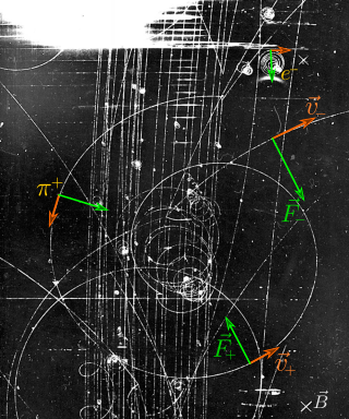
Magnetic field deflecting a charged particle, pseudo-defining magnetic rigidity for the particle.
In electromagnetism, a charged particle (of mass m and charge q) in a uniform magnetic field B is deflected by the field in a circular helical arc at velocity v and radius of curvaturer, where the helical trajectory inclined at an angle θ to B. The magnetic force is the centripetal force, so the force F acting on the particle is;
reducing to scalar form and solving for |B||r|;
serves as the definition for the magnetic rigidity of the particle.[13] Since this depends on the mass and charge of the particle, it is useful for determining the extent a particle deflects in a B field, which occurs experimentally in mass spectrometry and particle detectors.
↑ J.A. Wheeler; C. Misner; K.S. Thorne (1973). Gravitation. W.H. Freeman & Co. pp.72–73. ISBN0-7167-0344-0.. These authors use the Lorentz force in tensor form as definer of the electromagnetic tensorF, in turn the fields E and B.
In physics, the Lorentz force is the combination of electric and magnetic force on a point charge due to electromagnetic fields. A particle of charge q moving with a velocity v in an electric field E and a magnetic field B experiences a force of
Maxwell's equations, or Maxwell–Heaviside equations, are a set of coupled partial differential equations that, together with the Lorentz force law, form the foundation of classical electromagnetism, classical optics, and electric circuits. The equations provide a mathematical model for electric, optical, and radio technologies, such as power generation, electric motors, wireless communication, lenses, radar, etc. They describe how electric and magnetic fields are generated by charges, currents, and changes of the fields. The equations are named after the physicist and mathematician James Clerk Maxwell, who, in 1861 and 1862, published an early form of the equations that included the Lorentz force law. Maxwell first used the equations to propose that light is an electromagnetic phenomenon. The modern form of the equations in their most common formulation is credited to Oliver Heaviside.
Flux describes any effect that appears to pass or travel through a surface or substance. Flux is a concept in applied mathematics and vector calculus which has many applications to physics. For transport phenomena, flux is a vector quantity, describing the magnitude and direction of the flow of a substance or property. In vector calculus flux is a scalar quantity, defined as the surface integral of the perpendicular component of a vector field over a surface.
The electric potential is defined as the amount of work energy needed per unit of electric charge to move this charge from a reference point to the specific point in an electric field. More precisely, it is the energy per unit charge for a test charge that is so small that the disturbance of the field under consideration is negligible. The motion across the field is supposed to proceed with negligible acceleration, so as to avoid the test charge acquiring kinetic energy or producing radiation. By definition, the electric potential at the reference point is zero units. Typically, the reference point is earth or a point at infinity, although any point can be used.
In physics, Gauss's law, also known as Gauss's flux theorem, is a law relating the distribution of electric charge to the resulting electric field. In its integral form, it states that the flux of the electric field out of an arbitrary closed surface is proportional to the electric charge enclosed by the surface, irrespective of how that charge is distributed. Even though the law alone is insufficient to determine the electric field across a surface enclosing any charge distribution, this may be possible in cases where symmetry mandates uniformity of the field. Where no such symmetry exists, Gauss's law can be used in its differential form, which states that the divergence of the electric field is proportional to the local density of charge.
Hamiltonian mechanics emerged in 1833 as a reformulation of Lagrangian mechanics. Introduced by Sir William Rowan Hamilton, Hamiltonian mechanics replaces (generalized) velocities used in Lagrangian mechanics with (generalized) momenta. Both theories provide interpretations of classical mechanics and describe the same physical phenomena.
Electrostatics is a branch of physics that studies slow-moving or stationary electric charges.
Classical electromagnetism or classical electrodynamics is a branch of theoretical physics that studies the interactions between electric charges and currents using an extension of the classical Newtonian model; It is, therefore, a classical field theory. The theory provides a description of electromagnetic phenomena whenever the relevant length scales and field strengths are large enough that quantum mechanical effects are negligible. For small distances and low field strengths, such interactions are better described by quantum electrodynamics, which is a quantum field theory.
In electromagnetism, the magnetic moment is the magnetic strength and orientation of a magnet or other object that produces a magnetic field, expressed as a vector. Examples of objects that have magnetic moments include loops of electric current, permanent magnets, elementary particles, composite particles, various molecules, and many astronomical objects.
In electromagnetism, displacement current density is the quantity ∂D/∂t appearing in Maxwell's equations that is defined in terms of the rate of change of D, the electric displacement field. Displacement current density has the same units as electric current density, and it is a source of the magnetic field just as actual current is. However it is not an electric current of moving charges, but a time-varying electric field. In physical materials, there is also a contribution from the slight motion of charges bound in atoms, called dielectric polarization.
In classical electromagnetism, polarization density is the vector field that expresses the density of permanent or induced electric dipole moments in a dielectric material. When a dielectric is placed in an external electric field, its molecules gain electric dipole moment and the dielectric is said to be polarized. The electric dipole moment induced per unit volume of the dielectric material is called the electric polarization of the dielectric.
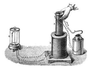
Faraday's law of induction is a basic law of electromagnetism predicting how a magnetic field will interact with an electric circuit to produce an electromotive force (emf)—a phenomenon known as electromagnetic induction. It is the fundamental operating principle of transformers, inductors, and many types of electric motors, generators and solenoids.
In physics, circulation is the line integral of a vector field around a closed curve. In fluid dynamics, the field is the fluid velocity field. In electrodynamics, it can be the electric or the magnetic field.
In physics and mathematics, in the area of vector calculus, Helmholtz's theorem, also known as the fundamental theorem of vector calculus, states that any sufficiently smooth, rapidly decaying vector field in three dimensions can be resolved into the sum of an irrotational (curl-free) vector field and a solenoidal (divergence-free) vector field; this is known as the Helmholtz decomposition or Helmholtz representation. It is named after Hermann von Helmholtz.
In classical electromagnetism, magnetic vector potential is the vector quantity defined so that its curl is equal to the magnetic field: . Together with the electric potential φ, the magnetic vector potential can be used to specify the electric field E as well. Therefore, many equations of electromagnetism can be written either in terms of the fields E and B, or equivalently in terms of the potentials φ and A. In more advanced theories such as quantum mechanics, most equations use potentials rather than fields.
A classical field theory is a physical theory that predicts how one or more physical fields interact with matter through field equations, without considering effects of quantization; theories that incorporate quantum mechanics are called quantum field theories. In most contexts, 'classical field theory' is specifically intended to describe electromagnetism and gravitation, two of the fundamental forces of nature.
The Vlasov equation is a differential equation describing time evolution of the distribution function of plasma consisting of charged particles with long-range interaction, such as the Coulomb interaction. The equation was first suggested for the description of plasma by Anatoly Vlasov in 1938 and later discussed by him in detail in a monograph.
In quantum mechanics, the probability current is a mathematical quantity describing the flow of probability. Specifically, if one thinks of probability as a heterogeneous fluid, then the probability current is the rate of flow of this fluid. It is a real vector that changes with space and time. Probability currents are analogous to mass currents in hydrodynamics and electric currents in electromagnetism. As in those fields, the probability current is related to the probability density function via a continuity equation. The probability current is invariant under gauge transformation.
In physics, Lagrangian mechanics is a formulation of classical mechanics founded on the stationary-action principle. It was introduced by the Italian-French mathematician and astronomer Joseph-Louis Lagrange in his 1788 work, Mécanique analytique.
Lagrangian field theory is a formalism in classical field theory. It is the field-theoretic analogue of Lagrangian mechanics. Lagrangian mechanics is used to analyze the motion of a system of discrete particles each with a finite number of degrees of freedom. Lagrangian field theory applies to continua and fields, which have an infinite number of degrees of freedom.
This page is based on this Wikipedia article Text is available under the CC BY-SA 4.0 license; additional terms may apply. Images, videos and audio are available under their respective licenses.