Diagram of factors that determine climate sensitivity. After increasing CO2 levels, there is an initial warming. This warming gets amplified by the net effect of climate feedbacks.
Climate sensitivity is a key measure in climate science and describes how much Earth's surface will warm in response to a doubling of the atmospheric carbon dioxide (CO2) concentration.[1][2] Its formal definition is: "The change in the surface temperature in response to a change in the atmospheric carbon dioxide (CO2) concentration or other radiative forcing."[3]:2223 This concept helps scientists understand the extent and magnitude of the effects of climate change.
Scientists do not know exactly how strong these climate feedbacks are. Therefore, it is difficult to predict the precise amount of warming that will result from a given increase in greenhouse gas concentrations. If climate sensitivity turns out to be on the high side of scientific estimates, the Paris Agreement goal of limiting global warming to below 2°C (3.6°F) will be even more difficult to achieve.[4]
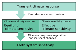
There are two main kinds of climate sensitivity: the transient climate response is the initial rise in global temperature when CO2 levels double, and the equilibrium climate sensitivity is the larger long-term temperature increase after the planet adjusts to the doubling. Climate sensitivity is estimated by several methods: looking directly at temperature and greenhouse gas concentrations since the Industrial Revolution began around the 1750s, using indirect measurements from the Earth's distant past, and simulating the climate.
Fundamentals
The rate at which energy reaches Earth (as sunlight) and leaves Earth (as heat radiation to space) must balance, or the planet will get warmer or cooler. An imbalance between incoming and outgoing radiation energy is called radiative forcing. A warmer planet radiates heat to space faster and so a new balance is eventually reached, with a higher temperature and stored energy content. However, the warming of the planet also has knock-on effects, which create further warming in an exacerbating feedback loop. Climate sensitivity is a measure of how much temperature change a given amount of radiative forcing will cause.[5]
Radiative forcings are generally quantified as Watts per square meter (W/m2) and averaged over Earth's uppermost surface defined as the top of the atmosphere.[6] The magnitude of a forcing is specific to the physical driver and is defined relative to an accompanying time span of interest for its application.[7] In the context of a contribution to long-term climate sensitivity from 1750 to 2020, the 50% increase in atmospheric CO 2 is characterized by a forcing of about +2.1W/m2.[8] In the context of shorter-term contributions to Earth's energy imbalance (i.e. its heating/cooling rate), time intervals of interest may be as short as the interval between measurement or simulation data samplings, and are thus likely to be accompanied by smaller forcing values. Forcings from such investigations have also been analyzed and reported at decadal time scales.[9][10]
Radiative forcing leads to long-term changes in global temperature.[11] A number of factors contribute radiative forcing: increased downwelling radiation from the greenhouse effect, variability in solar radiation from changes in planetary orbit, changes in solar irradiance, direct and indirect effects caused by aerosols (for example changes in albedo from cloud cover), and changes in land use (deforestation or the loss of reflective ice cover).[6] In contemporary research, radiative forcing by greenhouse gases is well understood. As of 2019[update], large uncertainties remain for aerosols.[12][13]
Carbon dioxide (CO2) levels rose from 280 parts per million (ppm) in the 18th century, when humans in the Industrial Revolution started burning significant amounts of fossil fuel such as coal, to over 415 ppm by 2020. As CO2 is a greenhouse gas, it hinders heat energy from leaving the Earth's atmosphere. In 2016, atmospheric CO2 levels had increased by 45% over preindustrial levels, and radiative forcing caused by increased CO2 was already more than 50% higher than in pre-industrial times because of non-linear effects.[14][note 1] Between the 18th-century start of the Industrial Revolution and the year 2020, the Earth's temperature rose by a little over one degree Celsius (about two degrees Fahrenheit).[15]
Societal importance
Because the economics of climate change mitigation depend greatly on how quickly carbon neutrality needs to be achieved, climate sensitivity estimates can have important economic and policy-making implications. One study suggests that halving the uncertainty of the value for transient climate response (TCR) could save trillions of dollars.[16] A higher climate sensitivity would mean more dramatic increases in temperature, which makes it more prudent to take significant climate action.[17] If climate sensitivity turns out to be on the high end of what scientists estimate, the Paris Agreement goal of limiting global warming to well below 2°C cannot be achieved, and temperature increases will exceed that limit, at least temporarily. One study estimated that emissions cannot be reduced fast enough to meet the 2°C goal if equilibrium climate sensitivity (the long-term measure) is higher than 3.4°C (6.1°F).[4] The more sensitive the climate system is to changes in greenhouse gas concentrations, the more likely it is to have decades when temperatures are much higher or much lower than the longer-term average.[18][19]
Factors that determine sensitivity
The radiative forcing caused by a doubling of atmospheric CO2 levels (from the pre-industrial 280 ppm) is approximately 3.7 watts per square meter (W/m2). In the absence of feedbacks, the energy imbalance would eventually result in roughly 1°C (1.8°F) of global warming. That figure is straightforward to calculate by using the Stefan–Boltzmann law[note 2][20] and is undisputed.[21]
A further contribution arises from climate feedbacks, both self-reinforcing and balancing.[22][23] The uncertainty in climate sensitivity estimates is mostly from the feedbacks in the climate system, including water vapour feedback, ice–albedo feedback, cloud feedback, and lapse rate feedback.[21] Balancing feedbacks tend to counteract warming by increasing the rate at which energy is radiated to space from a warmer planet. Self-reinfocing feedbacks increase warming; for example, higher temperatures can cause ice to melt, which reduces the ice area and the amount of sunlight the ice reflects, which in turn results in less heat energy being radiated back into space. The reflectiveness of a surface is called albedo. Climate sensitivity depends on the balance between those feedbacks.[20]
Types
Schematic of how different measures of climate sensitivity relate to one another
Depending on the time scale, there are two main ways to define climate sensitivity: the short-term transient climate response (TCR) and the long-term equilibrium climate sensitivity (ECS), both of which incorporate the warming from exacerbating feedback loops. They are not discrete categories, but they overlap. Sensitivity to atmospheric CO2 increases is measured in the amount of temperature change for doubling in the atmospheric CO2 concentration.[24][25]
Although the term "climate sensitivity" is usually used for the sensitivity to radiative forcing caused by rising atmospheric CO2, it is a general property of the climate system. Other agents can also cause a radiative imbalance. Climate sensitivity is the change in surface air temperature per unit change in radiative forcing, and the climate sensitivity parameter[note 3] is therefore expressed in units of °C/(W/m2). Climate sensitivity is approximately the same whatever the reason for the radiative forcing (such as from greenhouse gases or solar variation).[26] When climate sensitivity is expressed as the temperature change for a level of atmospheric CO2 double the pre-industrial level, its units are degrees Celsius (°C).
The transient climate response (TCR) is defined as "the change in the global mean surface temperature, averaged over a 20-year period, centered at the time of atmospheric carbon dioxide doubling, in a climate model simulation" in which the atmospheric CO2 concentration increases at 1% per year.[27] That estimate is generated by using shorter-term simulations.[28] The transient response is lower than the equilibrium climate sensitivity because slower feedbacks, which exacerbate the temperature increase, take more time to respond in full to an increase in the atmospheric CO2 concentration. For instance, the deep ocean takes many centuries to reach a new steady state after a perturbation during which it continues to serve as heatsink, which cools the upper ocean.[29] The IPCC literature assessment estimates that the TCR likely lies between 1°C (1.8°F) and 2.5°C (4.5°F).[30]
A related measure is the transient climate response to cumulative carbon emissions (TCRE), which is the globally averaged surface temperature change after 1000 GtC of CO2 has been emitted.[31] As such, it includes not only temperature feedbacks to forcing but also the carbon cycle and carbon cycle feedbacks.[32]
Equilibrium climate sensitivity
The equilibrium climate sensitivity (ECS) is the long-term temperature rise (equilibrium global mean near-surface air temperature) that is expected to result from a doubling of the atmospheric CO2 concentration (ΔT2×). It is a prediction of the new global mean near-surface air temperature once the CO2 concentration has stopped increasing, and most of the feedbacks have had time to have their full effect. Reaching an equilibrium temperature can take centuries or even millennia after CO2 has doubled. ECS is higher than TCR because of the oceans' short-term buffering effects.[25] Computer models are used for estimating the ECS.[33] A comprehensive estimate means that modelling the whole time span during which significant feedbacks continue to change global temperatures in the model, such as fully-equilibrating ocean temperatures, requires running a computer model that covers thousands of years. There are, however, less computing-intensive methods.[34]
The IPCC Sixth Assessment Report (AR6) stated that there is high confidence that ECS is within the range of 2.5°C to 4°C, with a best estimate of 3°C.[35]
The long time scales involved with ECS make it arguably a less relevant measure for policy decisions around climate change.[36]
Effective climate sensitivity
A common approximation to ECS is the effective equilibrium climate sensitivity, is an estimate of equilibrium climate sensitivity by using data from a climate system in model or real-world observations that is not yet in equilibrium.[27] Estimates assume that the net amplification effect of feedbacks, as measured after some period of warming, will remain constant afterwards.[37] That is not necessarily true, as feedbacks can change with time.[38][27] In many climate models, feedbacks become stronger over time and so the effective climate sensitivity is lower than the real ECS.[39]
Earth system sensitivity
By definition, equilibrium climate sensitivity does not include feedbacks that take millennia to emerge, such as long-term changes in Earth's albedo because of changes in ice sheets and vegetation. It also does not include the slow response of the deep oceans' warming, which takes millennia.[40] Earth system sensitivity (ESS) incorporates the effects of these slower feedback loops, such as the change in Earth's albedo from the melting of large continental ice sheets, which covered much of the Northern Hemisphere during the Last Glacial Maximum and still cover Greenland and Antarctica. Changes in albedo as a result of changes in vegetation, as well as changes in ocean circulation, are also included.[41][42] The longer-term feedback loops make the ESS larger than the ECS, possibly twice as large. Data from the geological history of Earth is used in estimating ESS. Differences between modern and long-ago climatic conditions mean that estimates of the future ESS are highly uncertain.[43] The carbon cycle is not included in the definition of the ESS, but all other elements of the climate system are included.[44]
Sensitivity to nature of forcing
Different forcing agents, such as greenhouse gases and aerosols, can be compared using their radiative forcing, the initial radiative imbalance averaged over the entire globe. Climate sensitivity is the amount of warming per radiative forcing. To a first approximation, the cause of the radiative imbalance does not matter. However, radiative forcing from sources other than CO2 can cause slightly more or less surface warming than the same averaged forcing from CO2. The amount of feedback varies mainly because the forcings are not uniformly distributed over the globe. Forcings that initially warm the Northern Hemisphere, land, or polar regions generate more self-reinforcing feedbacks (such as the ice-albedo feedback) than an equivalent forcing from CO2, which is more uniformly distributed over the globe. This gives rise to more overall warming. Several studies indicate that human-emitted aerosols are more effective than CO2 at changing global temperatures, and volcanic forcing is less effective.[45] When climate sensitivity to CO2 forcing is estimated using historical temperature and forcing (caused by a mix of aerosols and greenhouse gases), and that effect is not taken into account, climate sensitivity is underestimated.[46]
State dependence
Artist impression of a Snowball Earth.
Climate sensitivity has been defined as the short- or long-term temperature change resulting from any doubling of CO2, but there is evidence that the sensitivity of Earth's climate system is not constant. For instance, the planet has polar ice and high-altitude glaciers. Until the world's ice has completely melted, a self-reinforcing ice–albedo feedback loop makes the system more sensitive overall.[47] Throughout Earth's history, multiple periods are thought to have snow and ice cover almost the entire globe. In most models of "Snowball Earth", parts of the tropics were at least intermittently free of ice cover. As the ice advanced or retreated, climate sensitivity must have been very high, as the large changes in area of ice cover would have made for a very strong ice–albedo feedback. Volcanic atmospheric composition changes are thought to have provided the radiative forcing needed to escape the snowball state.[48]
Equilibrium climate sensitivity can change with climate.
Throughout the Quaternary period (the most recent 2.58million years), climate has oscillated between glacial periods, the most recent one being the Last Glacial Maximum, and interglacial periods, the most recent one being the current Holocene, but the period's climate sensitivity is difficult to determine. The Paleocene–Eocene Thermal Maximum, about 55.5million years ago, was unusually warm and may have been characterized by above-average climate sensitivity.[48]
Climate sensitivity may further change if tipping points are crossed. It is unlikely that tipping points will cause short-term changes in climate sensitivity. If a tipping point is crossed, climate sensitivity is expected to change at the time scale of the subsystem that hits its tipping point. Especially if there are multiple interacting tipping points, the transition of climate to a new state may be difficult to reverse.[49]
The two most common definitions of climate sensitivity specify the climate state: the ECS and the TCR are defined for a doubling with respect to the CO2 levels in the pre-industrial era. Because of potential changes in climate sensitivity, the climate system may warm by a different amount after a second doubling of CO2 from after a first doubling. The effect of any change in climate sensitivity is expected to be small or negligible in the first century after additional CO2 is released into the atmosphere.[47]
Estimation
Using Industrial Age (1750–present) data
Climate sensitivity can be estimated using the observed temperature increase, the observed ocean heat uptake, and the modelled or observed radiative forcing. The data are linked through a simple energy-balance model to calculate climate sensitivity.[50] Radiative forcing is often modelled because Earth observation satellites measuring it has existed during only part of the Industrial Age (only since the late 1950s). Estimates of climate sensitivity calculated by using these global energy constraints have consistently been lower than those calculated by using other methods,[51] around 2°C (3.6°F) or lower.[50][52][53][54]
Estimates of transient climate response (TCR) that have been calculated from models and observational data can be reconciled if it is taken into account that fewer temperature measurements are taken in the polar regions, which warm more quickly than the Earth as a whole. If only regions for which measurements are available are used in evaluating the model, the differences in TCR estimates are negligible.[25][55]
A very simple climate model could estimate climate sensitivity from Industrial Age data[21] by waiting for the climate system to reach equilibrium and then by measuring the resulting warming, ΔTeq (°C). Computation of the equilibrium climate sensitivity, S (°C), using the radiative forcing ΔF (W/m2) and the measured temperature rise, would then be possible. The radiative forcing resulting from a doubling of CO2, F2×CO2, is relatively well known, at about 3.7 W/m2. Combining that information results in this equation:
.
However, the climate system is not in equilibrium since the actual warming lags the equilibrium warming, largely because the oceans take up heat and will take centuries or millennia to reach equilibrium.[21] Estimating climate sensitivity from Industrial Age data requires an adjustment to the equation above. The actual forcing felt by the atmosphere is the radiative forcing minus the ocean's heat uptake, H (W/m2) and so climate sensitivity can be estimated:
The global temperature increase between the beginning of the Industrial Period, which is (taken as 1750, and 2011 was about 0.85°C (1.53°F). In 2011, the radiative forcing from CO2 and other long-lived greenhouse gases (mainly methane, nitrous oxide, and chlorofluorocarbon) that have been emitted since the 18th century was roughly 2.8 W/m2. The climate forcing, ΔF, also contains contributions from solar activity (+0.05 W/m2), aerosols (−0.9 W/m2), ozone (+0.35 W/m2), and other smaller influences, which brings the total forcing over the Industrial Period to 2.2 W/m2, according to the best estimate of the IPCC Fifth Assessment Report in 2014, with substantial uncertainty.[56] The ocean heat uptake, estimated by the same report to be 0.42 W/m2,[57] yields a value for S of 1.8°C (3.2°F).
Other strategies
In theory, Industrial Age temperatures could also be used to determine a time scale for the temperature response of the climate system and thus climate sensitivity:[58] if the effective heat capacity of the climate system is known, and the timescale is estimated using autocorrelation of the measured temperature, an estimate of climate sensitivity can be derived. In practice, however, the simultaneous determination of the time scale and heat capacity is difficult.[59][60][61]
Attempts have been made to use the 11-year solar cycle to constrain the transient climate response.[62]Solar irradiance is about 0.9 W/m2 higher during a solar maximum than during a solar minimum, and those effect can be observed in measured average global temperatures from 1959 to 2004.[63] Unfortunately, the solar minima in the period coincided with volcanic eruptions, which have a cooling effect on the global temperature. Because the eruptions caused a larger and less well-quantified decrease in radiative forcing than the reduced solar irradiance, it is questionable whether useful quantitative conclusions can be derived from the observed temperature variations.[64]
Observations of volcanic eruptions have also been used to try to estimate climate sensitivity, but as the aerosols from a single eruption last at most a couple of years in the atmosphere, the climate system can never come close to equilibrium, and there is less cooling than there would be if the aerosols stayed in the atmosphere for longer. Therefore, volcanic eruptions give information only about a lower bound on transient climate sensitivity.[65]
Using data from Earth's past
Historical climate sensitivity can be estimated by using reconstructions of Earth's past temperatures and CO2 levels. Paleoclimatologists have studied different geological periods, such as the warm Pliocene (5.3 to 2.6million years ago)[66] and the colder Pleistocene (2.6million to 11,700 years ago),[67] and sought periods that are in some way analogous to or informative about current climate change. Climates further back in Earth's history are more difficult to study because fewer data are available about them. For instance, past CO2 concentrations can be derived from air trapped in ice cores, but as of 2020[update], the oldest continuous ice core is less than one million years old.[68] Recent periods, such as the Last Glacial Maximum (LGM) (about 21,000 years ago) and the Mid-Holocene (about 6,000 years ago), are often studied, especially when more information about them becomes available.[69][70][71]
A 2007 estimate of sensitivity made using data from the most recent 420million years is consistent with sensitivities of current climate models and with other determinations.[72] The Paleocene–Eocene Thermal Maximum (about 55.5million years ago), a 20,000-year period during which massive amount of carbon entered the atmosphere and average global temperatures increased by approximately 6°C (11°F), also provides a good opportunity to study the climate system when it was in a warm state.[73] Studies of the last 800,000 years have concluded that climate sensitivity was greater in glacial periods than in interglacial periods.[74]
As the name suggests, the Last Glacial Maximum was much colder than today, and good data on atmospheric CO2 concentrations and radiative forcing from that period are available.[75] The period's orbital forcing was different from today's but had little direct effect on mean annual temperatures.[76] Estimating climate sensitivity from the Last Glacial Maximum can be done by several different ways.[75] One way is to use estimates of global radiative forcing and temperature directly. The set of feedback mechanisms active during the period, however, may be different from the feedbacks caused by a present doubling of CO2,[77] and such feedback differences across climate states must be accounted for when inferring today's climate sensitivity from paleoclimate evidence.[78][76][79] In a different approach, a model of intermediate complexity is used to simulate conditions during the period. Several versions of this single model are run, with different values chosen for uncertain parameters, such that each version has a different ECS. Outcomes that best simulate the LGM's observed cooling probably produce the most realistic ECS values.[80]
Using climate models
Frequency distribution of equilibrium climate sensitivity based on simulations of the doubling of CO2. Each model simulation has different estimates for processes which scientists do not sufficiently understand. Few of the simulations result in less than 2°C (3.6°F) of warming or significantly more than 4°C (7.2°F). However, the positive skew, which is also found in other studies, suggests that if carbon dioxide concentrations double, the probability of large or very large increases in temperature is greater than the probability of small increases.
Climate models simulate the CO2-driven warming of the future as well as the past. They operate on principles similar to those underlying models that predict the weather, but they focus on longer-term processes. Climate models typically begin with a starting state and then apply physical laws and knowledge about biology to predict future states. As with weather modelling, no computer has the power to model the complexity of the entire planet and simplifications are used to reduce that complexity to something manageable. An important simplification divides Earth's atmosphere into model cells. For instance, the atmosphere might be divided into cubes of air ten or one hundred kilometers on each side. Each model cell is treated as if it were homogeneous (uniform). Calculations for model cells are much faster than trying to simulate each molecule of air separately.[83]
A lower model resolution (large model cells and long time steps) takes less computing power but cannot simulate the atmosphere in as much detail. A model cannot simulate processes smaller than the model cells or shorter-term than a single time step. The effects of the smaller-scale and shorter-term processes must therefore be estimated by using other methods. Physical laws contained in the models may also be simplified to speed up calculations. The biosphere must be included in climate models. The effects of the biosphere are estimated by using data on the average behaviour of the average plant assemblage of an area under the modelled conditions. Climate sensitivity is therefore an emergent property of these models; it is not prescribed, but it follows from the interaction of all the modelled processes.[25]
To estimate climate sensitivity, a model is run by using a variety of radiative forcings (doubling quickly, doubling gradually, or following historical emissions) and the temperature results are compared to the forcing applied. Different models give different estimates of climate sensitivity, but they tend to fall within a similar range, as described above.
Testing, comparisons, and climate ensembles
Modelling of the climate system can lead to a wide range of outcomes. Models are often run that use different plausible parameters in their approximation of physical laws and the behaviour of the biosphere, which forms a perturbed physics ensemble, which attempts to model the sensitivity of the climate to different types and amounts of change in each parameter. Alternatively, structurally-different models developed at different institutions are put together, creating an ensemble. By selecting only the simulations that can simulate some part of the historical climate well, a constrained estimate of climate sensitivity can be made. One strategy for obtaining more accurate results is placing more emphasis on climate models that perform well in general.[84]
A model is tested using observations, paleoclimate data, or both to see if it replicates them accurately. If it does not, inaccuracies in the physical model and parametrizations are sought, and the model is modified. For models used to estimate climate sensitivity, specific test metrics that are directly and physically linked to climate sensitivity are sought. Examples of such metrics are the global patterns of warming,[85] the ability of a model to reproduce observed relative humidity in the tropics and subtropics,[86] patterns of heat radiation,[87] and the variability of temperature around long-term historical warming.[88][89][90] Ensemble climate models developed at different institutions tend to produce constrained estimates of ECS that are slightly higher than 3°C (5.4°F). The models with ECS slightly above 3°C (5.4°F) simulate the above situations better than models with a lower climate sensitivity.[91]
Many projects and groups exist to compare and to analyse the results of multiple models. For instance, the Coupled Model Intercomparison Project (CMIP) has been running since the 1990s.[92]
Historical estimates
Svante Arrhenius in the 19th century was the first person to quantify global warming as a consequence of a doubling of the concentration of CO2. In his first paper on the matter, he estimated that global temperature would rise by around 5 to 6°C (9.0 to 10.8°F) if the quantity of CO2 was doubled. In later work, he revised that estimate to 4°C (7.2°F).[93] Arrhenius used Samuel Pierpont Langley's observations of radiation emitted by the full moon to estimate the amount of radiation that was absorbed by water vapour and by CO2. To account for water vapour feedback, he assumed that relative humidity would stay the same under global warming.[94][95]
The first calculation of climate sensitivity that used detailed measurements of absorption spectra, as well as the first calculation to use a computer for numerical integration of the radiative transfer through the atmosphere, was performed by Syukuro Manabe and Richard Wetherald in 1967.[96] Assuming constant humidity, they computed an equilibrium climate sensitivity of 2.3°C per doubling of CO2, which they rounded to 2°C, the value most often quoted from their work, in the abstract of the paper. The work has been called "arguably the greatest climate-science paper of all time"[97] and "the most influential study of climate of all time."[98]
A committee on anthropogenic global warming, convened in 1979 by the United States National Academy of Sciences and chaired by Jule Charney,[99] estimated equilibrium climate sensitivity to be 3°C (5.4°F), plus or minus 1.5°C (2.7°F). The Manabe and Wetherald estimate (2°C (3.6°F)), James E. Hansen's estimate of 4°C (7.2°F), and Charney's model were the only models available in 1979. According to Manabe, speaking in 2004, "Charney chose 0.5°C as a reasonable margin of error, subtracted it from Manabe's number, and added it to Hansen's, giving rise to the 1.5 to 4.5°C (2.7 to 8.1°F) range of likely climate sensitivity that has appeared in every greenhouse assessment since...."[100] In 2008, climatologist Stefan Rahmstorf said: "At that time [it was published], the [Charney report estimate's] range [of uncertainty] was on very shaky ground. Since then, many vastly improved models have been developed by a number of climate research centers around the world."[21]
Assessment reports of IPCC
Historical estimates of climate sensitivity from the IPCC assessments. The first three reports gave a qualitative likely range, and the fourth and the fifth assessment report formally quantified the uncertainty. The dark blue range is judged as being more than 66% likely.
Despite considerable progress in the understanding of Earth's climate system, assessments continued to report similar uncertainty ranges for climate sensitivity for some time after the 1979 Charney report.[103] The First Assessment Report of the Intergovernmental Panel on Climate Change (IPCC), published in 1990, estimated that equilibrium climate sensitivity to a doubling of CO2 lay between 1.5 and 4.5°C (2.7 and 8.1°F), with a "best guess in the light of current knowledge" of 2.5°C (4.5°F).[104] The report used models with simplified representations of ocean dynamics. The IPCC supplementary report, 1992, which used full-ocean circulation models, saw "no compelling reason to warrant changing" the 1990 estimate;[105] and the IPCC Second Assessment Report stated, "No strong reasons have emerged to change [these estimates],"[106] In the reports, much of the uncertainty around climate sensitivity was attributed to insufficient knowledge of cloud processes. The 2001 IPCC Third Assessment Report also retained this likely range.[107]
Authors of the 2007 IPCC Fourth Assessment Report[101] stated that confidence in estimates of equilibrium climate sensitivity had increased substantially since the Third Annual Report.[108] The IPCC authors concluded that ECS is very likely to be greater than 1.5°C (2.7°F) and likely to lie in the range 2 to 4.5°C (3.6 to 8.1°F), with a most likely value of about 3°C (5.4°F). The IPCC stated that fundamental physical reasons and data limitations prevent a climate sensitivity higher than 4.5°C (8.1°F) from being ruled out, but the climate sensitivity estimates in the likely range agreed better with observations and the proxy climate data.[108]
The 2013 IPCC Fifth Assessment Report reverted to the earlier range of 1.5 to 4.5°C (2.7 to 8.1°F) (with high confidence), because some estimates using industrial-age data came out low.[25] The report also stated that ECS is extremely unlikely to be less than 1°C (1.8°F) (high confidence), and it is very unlikely to be greater than 6°C (11°F) (medium confidence). Those values were estimated by combining the available data with expert judgement.[102]
In preparation for the 2021 IPCC Sixth Assessment Report, a new generation of climate models was developed by scientific groups around the world.[109][110] Across 27 global climate models, estimates of a higher climate sensitivity were produced. The values spanned 1.8 to 5.6°C (3.2 to 10.1°F) and exceeded 4.5°C (8.1°F) in 10 of them.[111][112] The estimates for equilibrium climate sensitivity changed from 3.2°C to 3.7°C and the estimates for the transient climate response from 1.8°C, to 2.0°C.[113] The cause of the increased ECS lies mainly in improved modelling of clouds. Temperature rises are now believed to cause sharper decreases in the number of low clouds, and fewer low clouds means more sunlight is absorbed by the planet and less reflected to space.[113][111][114][115]
Remaining deficiencies in the simulation of clouds may have led to overestimates,[116] as models with the highest ECS values were not consistent with observed warming.[117] A fifth of the models began to 'run hot', predicting that global warming would produce significantly higher temperatures than is considered plausible.[118][119] According to these models, known as hot models, average global temperatures in the worst-case scenario would rise by more than 5°C above preindustrial levels by 2100,[120] with a "catastrophic" impact on human society.[121] In comparison, empirical observations combined with physics models indicate that the "very likely" range is between 2.3 and 4.7°C. Models with a very high climate sensitivity are also known to be poor at reproducing known historical climate trends, such as warming over the 20th century or cooling during the last ice age.[119] For these reasons the predictions of hot models are considered implausible, and have been given less weight by the IPCC in 2022.[116]
↑The CO2 level in 2016 was 403 ppm, which is less than 50% higher than the pre-industrial CO2 concentration of 278 ppm. However, because increased concentrations have a progressively-smaller warming effect, the Earth was already more than halfway to doubling of radiative forcing caused by CO2.
↑The calculation is as follows. In equilibrium, the energy of incoming and outgoing radiation have to balance. The outgoing radiation is given by the Stefan–Boltzmann law: . When incoming radiation increases, the outgoing radiation and therefore temperature must increase as well. The temperature rise directly caused by the additional radiative forcing, because of the doubling of CO2 is then given by
.
Given an effective temperature of 255K (−18°C; −1°F), a constant lapse rate, the value of the Stefan–Boltzmann constant of 5.67 W/m2 K−4 and around 4 W/m2, the equation gives a climate sensitivity of a world without feedback of approximately 1 K.
↑Here, the IPCC definition is used. In some other sources, the climate sensitivity parameter is simply called the climate sensitivity. The inverse of this parameter, is called the climate feedback parameter and is expressed in (W/m2)/°C.
↑"Climate sensitivity: fact sheet"(PDF). Australian government. Department of the Environment. Archived(PDF) from the original on 12 February 2020. Retrieved 12 February 2020.
12Climate Change: The IPCC Scientific Assessment (1990), Report prepared for Intergovernmental Panel on Climate Change by Working Group I, Houghton JT, Jenkins GT, Ephraums JJ (eds.), chapter 2, Radiative Forcing of ClimateArchived 2018-08-08 at the Wayback Machine , pp. 41–68
↑National Research Council (2005). Radiative Forcing of Climate Change: Expanding the Concept and Addressing Uncertainties. The National Academic Press. doi:10.17226/11175. ISBN978-0-309-09506-8.
123Planton S (2013). "Annex III: Glossary"(PDF). In Stocker TF, Qin D, Plattner GK, Tignor M, Allen SK, Boschung J, Nauels A, Xia Y, Bex V, Midgley PM (eds.). Climate Change 2013: The Physical Science Basis. Contribution of Working Group I to the Fifth Assessment Report of the Intergovernmental Panel on Climate Change. Cambridge University Press. p.1451. Archived(PDF) from the original on 16 October 2021. Retrieved 30 April 2019.
↑"Archived copy"(PDF). Archived(PDF) from the original on 11 August 2021. Retrieved 13 August 2021.{{cite web}}: CS1 maint: archived copy as title (link)
↑von der Heydt AS, Köhler P, van de Wal RS, Dijkstra HA (2014). "On the state dependency of fast feedback processes in (paleo) climate sensitivity". Geophysical Research Letters. 41 (18): 6484–6492. arXiv:1403.5391. doi:10.1002/2014GL061121. ISSN1944-8007. S2CID53703955.
↑McSweeney, Robert; Hausfather, Zeke (15 January 2018). "Q&A: How do climate models work?". Carbon Brief. Archived from the original on 5 March 2019. Retrieved 7 March 2020.
↑"CMIP - History". pcmdi.llnl.gov. Program for Climate Model Diagnosis & Intercomparison. Archived from the original on 28 July 2020. Retrieved 6 March 2020.
12Solomon S, etal. "Technical summary"(PDF). Climate Change 2007: Working Group I: The Physical Science Basis. Box TS.1: Treatment of Uncertainties in the Working Group I Assessment. Archived(PDF) from the original on 30 March 2019. Retrieved 30 March 2019., in IPCC AR4 WG1 2007
↑Albritton DL, etal. (2001). "Technical Summary: F.3 Projections of Future Changes in Temperature". In Houghton JT, etal. (eds.). Climate Change 2001: The Scientific Basis. Contribution of Working Group I to the Third Assessment Report of the Intergovernmental Panel on Climate Change. Cambridge University Press. Archived from the original on 12 January 2012.
Stocker TF, Qin D, Plattner GK, Alexander LV, Allen SK, Bindoff NL, etal. (2013). "Technical Summary"(PDF). IPCC AR5 WG1 2013. pp.33–115. Archived(PDF) from the original on 20 December 2019. Retrieved 12 February 2020.
This page is based on this Wikipedia article Text is available under the CC BY-SA 4.0 license; additional terms may apply. Images, videos and audio are available under their respective licenses.