Aerosol

Not to be confused with aerosil.

This article is about a suspension of particulates in a gas. For details on atmospheric particulate matter, see particulates.

For the spray can, see Aerosol spray dispenser.

Mist and fog are aerosols

An aerosol is a suspension of fine solid particles or liquid droplets in air or another gas. ^[1] Aerosols can be generated from natural or human causes. The term aerosol commonly refers to the mixture of particulates in air, and not to the particulate matter alone. ^[2] Examples of natural aerosols are fog or mist, dust, forest exudates, and geyser steam. Examples of human caused aerosols include particulate air pollutants, mist from the discharge at hydroelectric dams, irrigation mist, perfume from atomizers, smoke, dust, sprayed pesticides, and medical treatments for respiratory illnesses. ^[3] When a person inhales the contents of a vape pen or e-cigarette, they are inhaling an aerosol, too. ^[4]

The liquid or solid particles in an aerosol have diameters typically less than 1 μm. Larger particles with a significant settling speed make the mixture a suspension, but the distinction is not clear-cut. In everyday language, aerosol often refers to a dispensing system that delivers a consumer product from a spray can.

Diseases can spread by means of small droplets in the breath, ^[5] sometimes called bioaerosols. ^[6] One example was the transmission of the virus that lead to the COVID-19 pandemic. ^[7]

Definitions

See also: Particulates

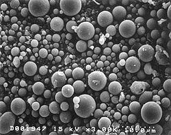
Photomicrograph made with a Scanning Electron Microscope (SEM): Fly ash particles at 2,000× magnification. Most of the particles in this aerosol are nearly spherical.

Aerosol spray can

Aerosol is defined as a suspension system of solid or liquid particles in a gas. An aerosol includes both the particles and the suspending gas, which is usually air. ^[1] Meteorologists usually refer them as particle matter - PM2.5 or PM10, depending on their size. ^[8] Frederick G. Donnan presumably first used the term aerosol during World War I to describe an aero-solution, clouds of microscopic particles in air. This term developed analogously to the term hydrosol, a colloid system with water as the dispersed medium. ^[9] Primary aerosols contain particles introduced directly into the gas; secondary aerosols form through gas-to-particle conversion. ^[10]

Key aerosol groups include sulfates, organic carbon, black carbon, nitrates, mineral dust, and sea salt, they usually clump together to form a complex mixture. ^[8] Various types of aerosol, classified according to physical form and how they were generated, include dust, fume, mist, smoke and fog. ^[11]

There are several measures of aerosol concentration. Environmental science and environmental health often use the mass concentration (M), defined as the mass of particulate matter per unit volume, in units such as μg/m³. Also commonly used is the number concentration (N), the number of particles per unit volume, in units such as number per m³ or number per cm³. ^[12]

Particle size has a major influence on particle properties, and the aerosol particle radius or diameter (d_p) is a key property used to characterise aerosols.

Aerosols vary in their dispersity. A monodisperse aerosol, producible in the laboratory, contains particles of uniform size. Most aerosols, however, as polydisperse colloidal systems, exhibit a range of particle sizes. ^[10] Liquid droplets are almost always nearly spherical, but scientists use an equivalent diameter to characterize the properties of various shapes of solid particles, some very irregular. The equivalent diameter is the diameter of a spherical particle with the same value of some physical property as the irregular particle. ^[13] The equivalent volume diameter (d_e) is defined as the diameter of a sphere of the same volume as that of the irregular particle. ^[14] Also commonly used is the aerodynamic diameter, d_a.

Generation and applications

People generate aerosols for various purposes, including:

• as test aerosols for calibrating instruments, performing research, and testing sampling equipment and air filters; ^[15]
• to deliver deodorants, paints, and other consumer products in sprays; ^[16]
• for dispersal and agricultural application
• for medical treatment of respiratory disease; ^[17] and
• in fuel injection systems and other combustion technology. ^[18]

Some devices for generating aerosols are: ^[3]

• Aerosol spray
• Atomizer nozzle or nebulizer
• Electrospray
• Electronic cigarette
• Vibrating orifice aerosol generator (VOAG)

In the atmosphere

Aerosol pollution over northern India and Bangladesh

Overview of large clouds of aerosols around Earth (green: smoke, blue: salt, yellow: dust, white: sulfuric)

Main article: Particulates

Several types of atmospheric aerosol have a significant effect on Earth's climate: volcanic, desert dust, sea-salt, that originating from biogenic sources and human-made. Volcanic aerosol forms in the stratosphere after an eruption as droplets of sulfuric acid that can prevail for up to two years, and reflect sunlight, lowering temperature. Desert dust, mineral particles blown to high altitudes, absorb heat and may be responsible for inhibiting storm cloud formation. Human-made sulfate aerosols, primarily from burning oil and coal, affect the behavior of clouds. ^[19]

Although all hydrometeors, solid and liquid, can be described as aerosols, a distinction is commonly made between such dispersions (i.e. clouds) containing activated drops and crystals, and aerosol particles. The atmosphere of Earth contains aerosols of various types and concentrations, including quantities of:

• natural inorganic materials: fine dust, sea salt, or water droplets
• natural organic materials: smoke, pollen, spores, or bacteria
• anthropogenic products of combustion such as: smoke, ashes or dusts

Aerosols can be found in urban ecosystems in various forms, for example:

• Dust
• Cigarette smoke
• Mist from aerosol spray cans
• Soot or fumes in car exhaust

The presence of aerosols in the Earth's atmosphere can influence its climate, as well as human health.

Effects

See also: Particulates § Climate effects

Aerosols have a cooling effect that is small compared to the radiative forcing (warming effect) of greenhouse gases.

• Volcanic eruptions release large amounts of sulphuric acid, hydrogen sulfide and hydrochloric acid into the atmosphere. These gases represent aerosols and eventually return to earth as acid rain, having a number of adverse effects on the environment and human life. ^[21]
• Aerosols interact with the Earth's energy budget in two ways, directly and indirectly.

E.g., a direct effect is that aerosols scatter and absorb incoming solar radiation. ^[22] This will mainly lead to a cooling of the surface (solar radiation is scattered back to space) but may also contribute to a warming of the surface (caused by the absorption of incoming solar energy). ^[23] This will be an additional element to the greenhouse effect and therefore contributing to the global climate change. ^[24]

The indirect effects refer to the aerosol interfering with formations that interact directly with radiation. For example, they are able to modify the size of the cloud particles in the lower atmosphere, thereby changing the way clouds reflect and absorb light and therefore modifying the Earth's energy budget. ^[21]

There is evidence to suggest that anthropogenic aerosols actually offset the effects of greenhouse gases in some areas, which is why the Northern Hemisphere shows slower surface warming than the Southern Hemisphere, although that just means that the Northern Hemisphere will absorb the heat later through ocean currents bringing warmer waters from the South. ^[25] On a global scale however, aerosol cooling decreases greenhouse-gases-induced heating without offsetting it completely. ^[26]

• When aerosols absorb pollutants, it facilitates the deposition of pollutants to the surface of the earth as well as to bodies of water. ^[24] This has the potential to be damaging to both the environment and human health.
• Aerosols in the 20 μm range show a particularly long persistence time in air conditioned rooms due to their "jet rider" behaviour (move with air jets, gravitationally fall out in slowly moving air); ^[27] as this aerosol size is most effectively adsorbed in the human nose, ^[28] the primordial infection site in COVID-19, such aerosols may contribute to the pandemic. ^[7]
• Aerosol particles with an effective diameter smaller than 10 μm can enter the bronchi, while the ones with an effective diameter smaller than 2.5 μm can enter as far as the gas exchange region in the lungs, ^[29] which can be hazardous to human health.

Size distribution

See also: Particulates § Size, shape, and solubility matter

The same hypothetical log-normal aerosol distribution plotted, from top to bottom, as a number vs. diameter distribution, a surface area vs. diameter distribution, and a volume vs. diameter distribution. Typical mode names are shown at the top. Each distribution is normalized so that the total area is 1000.

For a monodisperse aerosol, a single number—the particle diameter—suffices to describe the size of the particles. However, more complicated particle-size distributions describe the sizes of the particles in a polydisperse aerosol. This distribution defines the relative amounts of particles, sorted according to size. ^[30] One approach to defining the particle size distribution uses a list of the sizes of every particle in a sample. However, this approach proves tedious to ascertain in aerosols with millions of particles and awkward to use. Another approach splits the size range into intervals and finds the number (or proportion) of particles in each interval. These data can be presented in a histogram with the area of each bar representing the proportion of particles in that size bin, usually normalised by dividing the number of particles in a bin by the width of the interval so that the area of each bar is proportionate to the number of particles in the size range that it represents. ^[31] If the width of the bins tends to zero, the frequency function is: ^[32]

${\displaystyle \mathrm {d} f=f(d_{p})\,\mathrm {d} d_{p}}$

where

${\displaystyle d_{p}}$is the diameter of the particles

${\displaystyle \,\mathrm {d} f}$ is the fraction of particles having diameters between ${\displaystyle d_{p}}$ and ${\displaystyle d_{p}}$ + ${\displaystyle \mathrm {d} d_{p}}$

${\displaystyle f(d_{p})}$ is the frequency function

Therefore, the area under the frequency curve between two sizes a and b represents the total fraction of the particles in that size range: ^[32]

${\displaystyle f_{ab}=\int _{a}^{b}f(d_{p})\,\mathrm {d} d_{p}}$

It can also be formulated in terms of the total number density N: ^[33]

${\displaystyle dN=N(d_{p})\,\mathrm {d} d_{p}}$

Assuming spherical aerosol particles, the aerosol surface area per unit volume (S) is given by the second moment: ^[33]

${\displaystyle S=\pi /2\int _{0}^{\infty }N(d_{p})d_{p}^{2}\,\mathrm {d} d_{p}}$

And the third moment gives the total volume concentration (V) of the particles: ^[33]

${\displaystyle V=\pi /6\int _{0}^{\infty }N(d_{p})d_{p}^{3}\,\mathrm {d} d_{p}}$

The particle size distribution can be approximated. The normal distribution usually does not suitably describe particle size distributions in aerosols because of the skewness associated with a long tail of larger particles. Also for a quantity that varies over a large range, as many aerosol sizes do, the width of the distribution implies negative particles sizes, which is not physically realistic. However, the normal distribution can be suitable for some aerosols, such as test aerosols, certain pollen grains and spores. ^[34]

A more widely chosen log-normal distribution gives the number frequency as: ^[34]

${\displaystyle \mathrm {d} f={\frac {1}{d_{p}\sigma {\sqrt {2\pi }}}}e^{-{\frac {(ln(d_{p})-{\bar {d_{p}}})^{2}}{2\sigma ^{2}}}}\mathrm {d} d_{p}}$

where:

${\displaystyle \sigma }$ is the standard deviation of the size distribution and

${\displaystyle {\bar {d_{p}}}}$ is the arithmetic mean diameter.

The log-normal distribution has no negative values, can cover a wide range of values, and fits many observed size distributions reasonably well. ^[35]

Other distributions sometimes used to characterise particle size include: the Rosin-Rammler distribution, applied to coarsely dispersed dusts and sprays; the Nukiyama–Tanasawa distribution, for sprays of extremely broad size ranges; the power function distribution, occasionally applied to atmospheric aerosols; the exponential distribution, applied to powdered materials; and for cloud droplets, the Khrgian–Mazin distribution. ^[36]

Physics

Terminal velocity of a particle in a fluid

For low values of the Reynolds number (<1), true for most aerosol motion, Stokes' law describes the force of resistance on a solid spherical particle in a fluid. However, Stokes' law is only valid when the velocity of the gas at the surface of the particle is zero. For small particles (< 1 μm) that characterize aerosols, however, this assumption fails. To account for this failure, one can introduce the Cunningham correction factor, always greater than 1. Including this factor, one finds the relation between the resisting force on a particle and its velocity: ^[37]

${\displaystyle F_{D}={\frac {3\pi \eta Vd}{C_{c}}}}$

where

${\displaystyle F_{D}}$ is the resisting force on a spherical particle

${\displaystyle \eta }$ is the dynamic viscosity of the gas

${\displaystyle V}$ is the particle velocity

${\displaystyle C_{c}}$ is the Cunningham correction factor.

This allows us to calculate the terminal velocity of a particle undergoing gravitational settling in still air. Neglecting buoyancy effects, we find: ^[38]

${\displaystyle V_{TS}={\frac {\rho _{p}d^{2}gC_{c}}{18\eta }}}$

where

${\displaystyle V_{TS}}$ is the terminal settling velocity of the particle.

The terminal velocity can also be derived for other kinds of forces. If Stokes' law holds, then the resistance to motion is directly proportional to speed. The constant of proportionality is the mechanical mobility (B) of a particle: ^[39]

${\displaystyle B={\frac {V}{F_{D}}}={\frac {C_{c}}{3\pi \eta d}}}$

A particle traveling at any reasonable initial velocity approaches its terminal velocity exponentially with an e-folding time equal to the relaxation time: ^[40]

${\displaystyle V(t)=V_{f}-(V_{f}-V_{0})e^{-{\frac {t}{\tau }}}}$

where:

${\displaystyle V(t)}$ is the particle speed at time t

${\displaystyle V_{f}}$ is the final particle speed

${\displaystyle V_{0}}$ is the initial particle speed

To account for the effect of the shape of non-spherical particles, a correction factor known as the dynamic shape factor is applied to Stokes' law. It is defined as the ratio of the resistive force of the irregular particle to that of a spherical particle with the same volume and velocity: ^[14]

${\displaystyle \chi ={\frac {F_{D}}{3\pi \eta Vd_{e}}}}$

where:

${\displaystyle \chi }$ is the dynamic shape factor

Aerodynamic diameter

The aerodynamic diameter of an irregular particle is defined as the diameter of the spherical particle with a density of 1000 kg/m³ and the same settling velocity as the irregular particle. ^[41]

Neglecting the slip correction, the particle settles at the terminal velocity proportional to the square of the aerodynamic diameter, d_a: ^[41]

${\displaystyle V_{TS}={\frac {\rho _{0}d_{a}^{2}g}{18\eta }}}$

where

${\displaystyle \ \rho _{0}}$ = standard particle density (1000 kg/m³).

This equation gives the aerodynamic diameter: ^[42]

${\displaystyle d_{a}=d_{e}\left({\frac {\rho _{p}}{\rho _{0}\chi }}\right)^{\frac {1}{2}}}$

One can apply the aerodynamic diameter to particulate pollutants or to inhaled drugs to predict where in the respiratory tract such particles deposit. Pharmaceutical companies typically use aerodynamic diameter, not geometric diameter, to characterize particles in inhalable drugs. ^{[ citation needed ]}

Dynamics

The previous discussion focused on single aerosol particles. In contrast, aerosol dynamics explains the evolution of complete aerosol populations. The concentrations of particles will change over time as a result of many processes. External processes that move particles outside a volume of gas under study include diffusion, gravitational settling, and electric charges and other external forces that cause particle migration. A second set of processes internal to a given volume of gas include particle formation (nucleation), evaporation, chemical reaction, and coagulation. ^[43]

A differential equation called the Aerosol General Dynamic Equation (GDE) characterizes the evolution of the number density of particles in an aerosol due to these processes. ^[43]

${\displaystyle {\frac {\partial {n_{i}}}{\partial {t}}}=-\nabla \cdot n_{i}\mathbf {q} +\nabla \cdot D_{p}\nabla _{i}n_{i}+\left({\frac {\partial {n_{i}}}{\partial {t}}}\right)_{\mathrm {growth} }+\left({\frac {\partial {n_{i}}}{\partial {t}}}\right)_{\mathrm {coag} }-\nabla \cdot \mathbf {q} _{F}n_{i}}$

Change in time = Convective transport + brownian diffusion + gas-particle interactions + coagulation + migration by external forces

Where:

${\displaystyle n_{i}}$ is number density of particles of size category ${\displaystyle i}$

${\displaystyle \mathbf {q} }$ is the particle velocity

${\displaystyle D_{p}}$ is the particle Stokes-Einstein diffusivity

${\displaystyle \mathbf {q} _{F}}$ is the particle velocity associated with an external force

Coagulation

As particles and droplets in an aerosol collide with one another, they may undergo coalescence or aggregation. This process leads to a change in the aerosol particle-size distribution, with the mode increasing in diameter as total number of particles decreases. ^[44] On occasion, particles may shatter apart into numerous smaller particles; however, this process usually occurs primarily in particles too large for consideration as aerosols.

Dynamics regimes

The Knudsen number of the particle define three different dynamical regimes that govern the behaviour of an aerosol:

${\displaystyle K_{n}={\frac {2\lambda }{d}}}$

where ${\displaystyle \lambda }$ is the mean free path of the suspending gas and ${\displaystyle d}$ is the diameter of the particle. ^[45] For particles in the free molecular regime, K_n >> 1; particles small compared to the mean free path of the suspending gas. ^[46] In this regime, particles interact with the suspending gas through a series of "ballistic" collisions with gas molecules. As such, they behave similarly to gas molecules, tending to follow streamlines and diffusing rapidly through Brownian motion. The mass flux equation in the free molecular regime is:

${\displaystyle I={\frac {\pi a^{2}}{k_{b}}}\left({\frac {P_{\infty }}{T_{\infty }}}-{\frac {P_{A}}{T_{A}}}\right)\cdot C_{A}\alpha }$

where a is the particle radius, P_∞ and P_A are the pressures far from the droplet and at the surface of the droplet respectively, k_b is the Boltzmann constant, T is the temperature, C_A is mean thermal velocity and α is mass accommodation coefficient.^{[ citation needed ]} The derivation of this equation assumes constant pressure and constant diffusion coefficient.

Particles are in the continuum regime when K_n << 1. ^[46] In this regime, the particles are big compared to the mean free path of the suspending gas, meaning that the suspending gas acts as a continuous fluid flowing round the particle. ^[46] The molecular flux in this regime is:

${\displaystyle I_{cont}\sim {\frac {4\pi aM_{A}D_{AB}}{RT}}\left(P_{A\infty }-P_{AS}\right)}$

where a is the radius of the particle A, M_A is the molecular mass of the particle A, D_AB is the diffusion coefficient between particles A and B, R is the ideal gas constant, T is the temperature (in absolute units like kelvin), and P_A∞ and P_AS are the pressures at infinite and at the surface respectively.^{[ citation needed ]}

The transition regime contains all the particles in between the free molecular and continuum regimes or K_n ≈ 1. The forces experienced by a particle are a complex combination of interactions with individual gas molecules and macroscopic interactions. The semi-empirical equation describing mass flux is:

${\displaystyle I=I_{cont}\cdot {\frac {1+K_{n}}{1+1.71K_{n}+1.33{K_{n}}^{2}}}}$

where I_cont is the mass flux in the continuum regime.^{[ citation needed ]} This formula is called the Fuchs-Sutugin interpolation formula. These equations do not take into account the heat release effect.

Partitioning

Condensation and evaporation

Aerosol partitioning theory governs condensation on and evaporation from an aerosol surface, respectively. Condensation of mass causes the mode of the particle-size distributions of the aerosol to increase; conversely, evaporation causes the mode to decrease. Nucleation is the process of forming aerosol mass from the condensation of a gaseous precursor, specifically a vapor. Net condensation of the vapor requires supersaturation, a partial pressure greater than its vapor pressure. This can happen for three reasons:^{[ citation needed ]}

1. Lowering the temperature of the system lowers the vapor pressure.
2. Chemical reactions may increase the partial pressure of a gas or lower its vapor pressure.
3. The addition of additional vapor to the system may lower the equilibrium vapor pressure according to Raoult's law.

There are two types of nucleation processes. Gases preferentially condense onto surfaces of pre-existing aerosol particles, known as heterogeneous nucleation. This process causes the diameter at the mode of particle-size distribution to increase with constant number concentration. ^[47] With sufficiently high supersaturation and no suitable surfaces, particles may condense in the absence of a pre-existing surface, known as homogeneous nucleation. This results in the addition of very small, rapidly growing particles to the particle-size distribution. ^[47]

Activation

Water coats particles in aerosols, making them activated, usually in the context of forming a cloud droplet (such as natural cloud seeding by aerosols from trees in a forest). ^[48] Following the Kelvin equation (based on the curvature of liquid droplets), smaller particles need a higher ambient relative humidity to maintain equilibrium than larger particles do. The following formula gives relative humidity at equilibrium:

${\displaystyle RH={\frac {p_{s}}{p_{0}}}\times 100\%=S\times 100\%}$

where ${\displaystyle p_{s}}$ is the saturation vapor pressure above a particle at equilibrium (around a curved liquid droplet), p₀ is the saturation vapor pressure (flat surface of the same liquid) and S is the saturation ratio.

Kelvin equation for saturation vapor pressure above a curved surface is:

${\displaystyle \ln {p_{s} \over p_{0}}={\frac {2\sigma M}{RT\rho \cdot r_{p}}}}$

where r_p droplet radius, σ surface tension of droplet, ρ density of liquid, M molar mass, T temperature, and R molar gas constant.

Solution to the general dynamic equation

There are no general solutions to the general dynamic equation (GDE); ^[49] common methods used to solve the general dynamic equation include: ^[50]

• Moment method ^[51]
• Modal/sectional method, ^[52] and
• Quadrature method of moments ^{[53] [54]} /Taylor-series expansion method of moments, ^{[55] [56]} and
• Monte Carlo method. ^[57]

Detection

Aerosol can either be measured in-situ or with remote sensing techniques.

In situ observations

Some available in situ measurement techniques include:

• Aerosol mass spectrometer (AMS)
• Differential mobility analyzer (DMA)
• Electrical aerosol spectrometer (EAS)
• Aerodynamic particle sizer (APS)
• Aerodynamic aerosol classifier (AAC)
• Wide range particle spectrometer (WPS)
• Micro-Orifice Uniform Deposit Impactor(MOUDI)
• Condensation particle counter (CPC)
• Epiphaniometer
• Electrical low pressure impactor (ELPI)
• Aerosol particle mass-analyser (APM)
• Centrifugal Particle Mass Analyser (CPMA)

Remote sensing approach

Remote sensing approaches include:

• Sun photometer
• Lidar
• Imaging spectroscopy

Size selective sampling

Particles can deposit in the nose, mouth, pharynx and larynx (the head airways region), deeper within the respiratory tract (from the trachea to the terminal bronchioles), or in the alveolar region. ^[58] The location of deposition of aerosol particles within the respiratory system strongly determines the health effects of exposure to such aerosols. ^[58] This phenomenon led people to invent aerosol samplers that select a subset of the aerosol particles that reach certain parts of the respiratory system. ^[59]

Examples of these subsets of the particle-size distribution of an aerosol, important in occupational health, include the inhalable, thoracic, and respirable fractions. The fraction that can enter each part of the respiratory system depends on the deposition of particles in the upper parts of the airway. ^[60] The inhalable fraction of particles, defined as the proportion of particles originally in the air that can enter the nose or mouth, depends on external wind speed and direction and on the particle-size distribution by aerodynamic diameter. ^[61] The thoracic fraction is the proportion of the particles in ambient aerosol that can reach the thorax or chest region. ^[62] The respirable fraction is the proportion of particles in the air that can reach the alveolar region. ^[63] To measure the respirable fraction of particles in air, a pre-collector is used with a sampling filter. The pre-collector excludes particles as the airways remove particles from inhaled air. The sampling filter collects the particles for measurement. It is common to use cyclonic separation for the pre-collector, but other techniques include impactors, horizontal elutriators, and large pore membrane filters. ^[64]

Two alternative size-selective criteria, often used in atmospheric monitoring, are PM₁₀ and PM_2.5. PM₁₀ is defined by ISO as particles which pass through a size-selective inlet with a 50% efficiency cut-off at 10 μm aerodynamic diameter and PM_2.5 as particles which pass through a size-selective inlet with a 50% efficiency cut-off at 2.5 μm aerodynamic diameter. PM₁₀ corresponds to the "thoracic convention" as defined in ISO 7708:1995, Clause 6; PM_2.5 corresponds to the "high-risk respirable convention" as defined in ISO 7708:1995, 7.1. ^[65] The United States Environmental Protection Agency replaced the older standards for particulate matter based on Total Suspended Particulate with another standard based on PM₁₀ in 1987 ^[66] and then introduced standards for PM_2.5 (also known as fine particulate matter) in 1997. ^[67]

See also

• Aerogel
• Aeroplankton
• Aerosol transmission
• Bioaerosol
• Deposition (Aerosol physics)
• Global dimming
• Nebulizer
• Monoterpene
• Stratospheric aerosol injection

References

1. Hinds 1999, p. 3.
2. Seinfeld J, Pandis S (1998). Atmospheric Chemistry and Physics: From Air Pollution to Climate Change (2nd ed.). Hoboken, New Jersey: John Wiley & Sons. p.  97. ISBN   978-0-471-17816-3.
3. Hidy 1984, p. 254.
4. "Tobacco: E-cigarettes". www.who.int. Retrieved 2021-08-24.
5. Hunziker, Patrick (2021-10-01). "Minimising exposure to respiratory droplets, 'jet riders' and aerosols in air-conditioned hospital rooms by a 'Shield-and-Sink' strategy". BMJ Open. 11 (10): e047772. doi:10.1136/bmjopen-2020-047772. ISSN   2044-6055. PMC   8520596 . PMID   34642190.
6. Fuller, Joanna Kotcher (2017-01-31). Surgical Technology – E-Book: Principles and Practice. Elsevier Health Sciences. ISBN   978-0-323-43056-2.
7. McNeill VF (June 2022). "Airborne Transmission of SARS-CoV-2: Evidence and Implications for Engineering Controls". Annual Review of Chemical and Biomolecular Engineering. 13 (1): 123–140. doi:10.1146/annurev-chembioeng-092220-111631. PMID   35300517. S2CID   247520571.
8. "Aerosols: Tiny Particles, Big Impact". earthobservatory.nasa.gov. 2 November 2010.
9. Hidy 1984, p. 5.
10. Hinds 1999, p. 8.
11. Colbeck & Lazaridis 2014, p. Ch. 1.1.
12. Hinds 1999, pp. 10–11.
13. Hinds 1999, p. 10.
14. Hinds 1999, p. 51.
15. Hinds 1999, p. 428.
16. Hidy 1984, p. 255.
17. Hidy 1984, p. 274.
18. Hidy 1984, p. 278.
19. "Atmospheric Aerosols: What Are They, and Why Are They So Important?". NASA Langley Research Center. 22 Apr 2008. Retrieved 27 December 2014.
20. Forster, Piers M.; Smith, Christopher J.; Walsh, Tristram; Lamb, William F.; et al. (2023). "Indicators of Global Climate Change 2022: annual update of large-scale indicators of the state of the climate system and human influence" (PDF). Earth System Science Data. 15 (6). Copernicus Programme: 2295–2327. Bibcode:2023ESSD...15.2295F. doi: 10.5194/essd-15-2295-2023 . Fig. 2(a).
21. Allen, Bob. "Atmospheric Aerosols: What Are They, and Why Are They So Important?". NASA. Retrieved 8 July 2014.
22. Highwood, Ellie (2018-09-05). "Aerosols and Climate". Royal Meteorological Society. Retrieved 2019-10-07.
23. "Fifth Assessment Report - Climate Change 2013". www.ipcc.ch. Retrieved 2018-02-07.
24. Kommalapati, Raghava R.; Valsaraj, Kalliat T. (2009). Atmospheric aerosols: Characterization, chemistry, modeling, and climate. Vol. 1005. Washington, DC: American Chemical Society. pp. 1–10. doi:10.1021/bk-2009-1005.ch001. ISBN   978-0-8412-2482-7.
25. Anthropogenic Aerosols, Greenhouse Gases, and the Uptake, Transport, and Storage of Excess Heat in the Climate System Irving, D. B.; Wijffels, S.; Church, J. A. (2019). "Anthropogenic Aerosols, Greenhouse Gases, and the Uptake, Transport, and Storage of Excess Heat in the Climate System". Geophysical Research Letters. 46 (9): 4894–4903. Bibcode:2019GeoRL..46.4894I. doi: 10.1029/2019GL082015 . hdl: 1912/24327 .
26. GIEC AR6 WG1 - Figure SPM.2 https://www.ipcc.ch/report/sixth-assessment-report-working-group-i/
27. Hunziker, Patrick (2020-12-16). "Minimizing exposure to respiratory droplets, 'jet riders' and aerosols in air-conditioned hospital rooms by a 'Shield-and-Sink' strategy". medRxiv   10.1101/2020.12.08.20233056v1 .
28. Kesavanathan, Jana; Swift, David L. (1998). "Human Nasal Passage Particle Deposition: The Effect of Particle Size, Flow Rate, and Anatomical Factors". Aerosol Science and Technology. 28 (5): 457–463. Bibcode:1998AerST..28..457K. doi:10.1080/02786829808965537. ISSN   0278-6826.
29. Grainger, Don. "Volcanic Emissions". Earth Observation Data Group, Department of Physics, University of Oxford. University of Oxford. Retrieved 8 July 2014.
30. Jillavenkatesa, A; Dapkunas, SJ; Lin-Sien, Lum (2001). "Particle Size Characterization". NIST Special Publication. 960–1.
31. Hinds 1999, pp. 75–77.
32. Hinds 1999, p. 79.
33. Hidy 1984, p. 58.
34. Hinds 1999, p. 90.
35. Hinds 1999, p. 91.
36. Hinds 1999, pp. 104–5.
37. Hinds 1999, p. 44-49.
38. Hinds 1999, p. 49.
39. Hinds 1999, p. 47.
40. Hinds 1999, p. 115.
41. Hinds 1999, p. 53.
42. Hinds 1999, p. 54.
43. Hidy 1984, p. 60.
44. Hinds 1999, p. 260.
45. Baron, P. A. & Willeke, K. (2001). "Gas and Particle Motion". Aerosol Measurement: Principles, Techniques, and Applications.
46. DeCarlo, P.F. (2004). "Particle Morphology and Density Characterization by Combined Mobility and Aerodynamic Diameter Measurements. Part 1: Theory". Aerosol Science and Technology. 38 (12): 1185–1205. Bibcode:2004AerST..38.1185D. doi: 10.1080/027868290903907 .
47. Hinds 1999, p. 288.
48. Spracklen, Dominick V; Bonn, Boris; Carslaw, Kenneth S (2008-12-28). "Boreal forests, aerosols and the impacts on clouds and climate". Philosophical Transactions of the Royal Society A: Mathematical, Physical and Engineering Sciences. 366 (1885): 4613–4626. Bibcode:2008RSPTA.366.4613S. doi:10.1098/rsta.2008.0201. ISSN   1364-503X. PMID   18826917. S2CID   206156442.
49. Hidy 1984, p. 62.
50. Friedlander 2000.
51. Hulburt, H.M.; Katz, S. (1964). "Some problems in particle technology". Chemical Engineering Science. 19 (8): 555–574. doi:10.1016/0009-2509(64)85047-8.
52. Landgrebe, James D.; Pratsinis, Sotiris E. (1990). "A discrete-sectional model for particulate production by gas-phase chemical reaction and aerosol coagulation in the free-molecular regime". Journal of Colloid and Interface Science. 139 (1): 63–86. Bibcode:1990JCIS..139...63L. doi:10.1016/0021-9797(90)90445-T.
53. McGraw, Robert (1997). "Description of Aerosol Dynamics by the Quadrature Method of Moments". Aerosol Science and Technology. 27 (2): 255–265. Bibcode:1997AerST..27..255M. doi: 10.1080/02786829708965471 .
54. Marchisio, Daniele L.; Fox, Rodney O. (2005). "Solution of population balance equations using the direct quadrature method of moments". Journal of Aerosol Science . 36 (1): 43–73. Bibcode:2005JAerS..36...43M. doi:10.1016/j.jaerosci.2004.07.009.
55. Yu, Mingzhou; Lin, Jianzhong; Chan, Tatleung (2008). "A New Moment Method for Solving the Coagulation Equation for Particles in Brownian Motion". Aerosol Science and Technology. 42 (9): 705–713. Bibcode:2008AerST..42..705Y. doi:10.1080/02786820802232972. hdl: 10397/9612 . S2CID   120582575.
56. Yu, Mingzhou; Lin, Jianzhong (2009). "Taylor-expansion moment method for agglomerate coagulation due to Brownian motion in the entire size regime". Journal of Aerosol Science. 40 (6): 549–562. Bibcode:2009JAerS..40..549Y. doi:10.1016/j.jaerosci.2009.03.001.
57. Kraft, Murkus (2005). "Modelling of Particulate Processes". KONA Powder and Particle Journal. 23: 18–35. doi: 10.14356/kona.2005007 .
58. Hinds 1999, p. 233.
59. Hinds 1999, p. 249.
60. Hinds 1999, p. 244.
61. Hinds 1999, p. 246.
62. Hinds 1999, p. 254.
63. Hinds 1999, p. 250.
64. Hinds 1999, p. 252.
65. "Particulate pollution – PM10 and PM2.5". Recognition, Evaluation, Control. News and views from Diamond Environmental Limited. 2010-12-10. Retrieved 23 September 2012.
66. "Particulate Matter (PM-10)". Archived from the original on 1 September 2012. Retrieved 23 September 2012.
67. "Basic Information" . Retrieved 23 September 2012.

Sources

• Colbeck, Ian; Lazaridis, Mihalis, eds. (2014). Aerosol Science: Technology and Applications. John Wiley & Sons - Science. ISBN   978-1-119-97792-6.
• Friedlander, S. K. (2000). Smoke, Dust and Haze: Fundamentals of Aerosol Behavior (2nd ed.). New York: Oxford University Press. ISBN   0-19-512999-7.
• Hinds, William C. (1999). Aerosol Technology (2nd ed.). Wiley - Interscience. ISBN   978-0-471-19410-1.
• Hidy, George M. (1984). Aerosols, An Industrial and Environmental Science. Academic Press, Inc. ISBN   978-0-12-412336-6.

External links

• International Aerosol Research Assembly Archived 2020-01-21 at the Wayback Machine
• American Association for Aerosol Research
• NIOSH Manual of Analytical Methods (see chapters on aerosol sampling)