The existence of electron spin angular momentum is inferred from experiments, such as the Stern–Gerlach experiment, in which silver atoms were observed to possess two possible discrete angular momenta despite having no orbital angular momentum.[5] The existence of the electron spin can also be inferred theoretically from the spin–statistics theorem and from the Pauli exclusion principle—and vice versa, given the particular spin of the electron, one may derive the Pauli exclusion principle.
Spin is described mathematically as a vector for some particles such as photons, and as spinors and bispinors for other particles such as electrons. Spinors and bispinors behave similarly to vectors: they have definite magnitudes and change under rotations; however, they use an unconventional "direction". All elementary particles of a given kind have the same magnitude of spin angular momentum, though its direction may change. These are indicated by assigning the particle a spin quantum number.[2]
The SI unit of spin is the same as classical angular momentum (i.e., N·m·s, J·s, or kg·m2·s−1). In practice, spin is usually given as a dimensionless spin quantum number by dividing the spin angular momentum by the reduced Planck constantħ, which has the same dimensions as angular momentum. Often, the "spin quantum number" is simply called "spin".
Relation to classical rotation
Since elementary particles are point-like, self-rotation is not well-defined for them. However, spin implies that the phase of the particle depends on the angle as , for rotation of angle θ around the axis parallel to the spin S. This is equivalent to the quantum-mechanical interpretation of momentum as phase dependence in the position, and of orbital angular momentum as phase dependence in the angular position.
Photon spin is the quantum-mechanical description of light polarization, where spin+1 and spin−1 represent two opposite directions of circular polarization. Thus, light of a defined circular polarization consists of photons with the same spin, either all +1 or all −1. Spin represents polarization for other vector bosons as well.
For fermions, the picture is less clear. Angular velocity is equal by Ehrenfest theorem to the derivative of the Hamiltonian to its conjugate momentum, which is the total angular momentum operatorJ = L + S. Therefore, if the Hamiltonian H is dependent upon the spin S, dH/dS is non-zero, and the spin causes angular velocity, and hence actual rotation, i.e. a change in the phase-angle relation over time. However, whether this holds for free electron is ambiguous, since for an electron, S2 is constant, and therefore it is a matter of interpretation whether the Hamiltonian includes such a term. Nevertheless, spin appears in the Dirac equation, and thus the relativistic Hamiltonian of the electron, treated as a Dirac field, can be interpreted as including a dependence in the spin S.[6] Under this interpretation, free electrons also self-rotate, with the Zitterbewegung effect understood as this rotation.
As the name suggests, spin was originally conceived as the rotation of a particle around some axis. While spin obeys the same mathematical laws as quantizedangular momenta do, spin has some peculiar properties that distinguish it from orbital angular momenta:
Spin quantum numbers may take half-integer values.
Although the direction of its spin can be changed, the magnitude of the spin of an elementary particle cannot be changed.
The conventional definition of the spin quantum number is s = n/2, where n can be any non-negative integer. Hence the allowed values of s are 0, 1/2, 1, 3/2, 2, etc. The value of s for an elementary particle depends only on the type of particle and cannot be altered in any known way (in contrast to the spin direction described below). The spin angular momentum S of any physical system is quantized. The allowed values of S are
where h is the Planck constant, and is the reduced Planck constant. In contrast, orbital angular momentum can only take on integer values of s; i.e., even-numbered values of n.
Fermions and bosons
Those particles with half-integer spins, such as 1/2, 3/2, 5/2, are known as fermions, while those particles with integer spins, such as 0, 1, 2, are known as bosons. The two families of particles obey different rules and broadly have different roles in the world around us. A key distinction between the two families is that fermions obey the Pauli exclusion principle: that is, there cannot be two identical fermions simultaneously having the same quantum numbers (meaning, roughly, having the same position, velocity and spin direction). Fermions obey the rules of Fermi–Dirac statistics. In contrast, bosons obey the rules of Bose–Einstein statistics and have no such restriction, so they may "bunch together" in identical states. Also, composite particles can have spins different from their component particles. For example, a helium-4 atom in the ground state has spin0 and behaves like a boson, even though the quarks and electrons which make it up are all fermions.
This has some profound consequences:
Quarks and leptons (including electrons and neutrinos), which make up what is classically known as matter, are all fermions with spin1/2. The common idea that "matter takes up space" actually comes from the Pauli exclusion principle acting on these particles to prevent the fermions from being in the same quantum state. Further compaction would require electrons to occupy the same energy states, and therefore a kind of pressure (sometimes known as degeneracy pressure of electrons) acts to resist the fermions being overly close. Elementary fermions with other spins (3/2, 5/2, etc.) are not known to exist.
Elementary particles which are thought of as carrying forces are all bosons with spin1. They include the photon, which carries the electromagnetic force, the gluon (strong force), and the W and Z bosons (weak force). The ability of bosons to occupy the same quantum state is used in the laser, which aligns many photons having the same quantum number (the same direction and frequency), superfluidliquid helium resulting from helium-4 atoms being bosons, and superconductivity, where pairs of electrons (which individually are fermions) act as single composite bosons. Elementary bosons with other spins (0, 2, 3, etc.) were not historically known to exist, although they have received considerable theoretical treatment and are well established within their respective mainstream theories. In particular, theoreticians have proposed the graviton (predicted to exist by some quantum gravity theories) with spin2, and the Higgs boson (explaining electroweak symmetry breaking) with spin0. Since 2013, the Higgs boson with spin0 has been considered proven to exist.[7] It is the first scalar elementary particle (spin0) known to exist in nature.
Atomic nuclei have nuclear spin which may be either half-integer or integer, so that the nuclei may be either fermions or bosons.
The spin–statistics theorem splits particles into two groups: bosons and fermions, where bosons obey Bose–Einstein statistics, and fermions obey Fermi–Dirac statistics (and therefore the Pauli exclusion principle). Specifically, the theory states that particles with an integer spin are bosons, while all other particles have half-integer spins and are fermions. As an example, electrons have half-integer spin and are fermions that obey the Pauli exclusion principle, while photons have integer spin and do not. The theorem relies on both quantum mechanics and the theory of special relativity, and this connection between spin and statistics has been called "one of the most important applications of the special relativity theory".[8]
Schematic diagram depicting the spin of the neutron as the black arrow and magnetic field lines associated with the neutron magnetic moment. The neutron has a negative magnetic moment. While the spin of the neutron is upward in this diagram, the magnetic field lines at the center of the dipole are downward.
The intrinsic magnetic moment μ of a spin-1/2 particle with charge q, mass m, and spin angular momentum S, is[9]
where the dimensionless quantitygs is called the spin g-factor. For exclusively orbital rotations it would be 1 (assuming that the mass and the charge occupy spheres of equal radius).
The electron, being a charged elementary particle, possesses a nonzero magnetic moment. One of the triumphs of the theory of quantum electrodynamics is its accurate prediction of the electron g-factor, which has been experimentally determined to have the value −2.00231930436256(35), with the digits in parentheses denoting measurement uncertainty in the last two digits at one standard deviation.[10] The value of 2 arises from the Dirac equation, a fundamental equation connecting the electron's spin with its electromagnetic properties, and the deviation from −2 arises from the electron's interaction with the surrounding electromagnetic field, including its own field.[11]
Composite particles also possess magnetic moments associated with their spin. In particular, the neutron possesses a non-zero magnetic moment despite being electrically neutral. This fact was an early indication that the neutron is not an elementary particle. In fact, it is made up of quarks, which are electrically charged particles. The magnetic moment of the neutron comes from the spins of the individual quarks and their orbital motions.
Neutrinos are both elementary and electrically neutral. The minimally extended Standard Model that takes into account non-zero neutrino masses predicts neutrino magnetic moments of:[12][13][14]
where the μν are the neutrino magnetic moments, mν are the neutrino masses, and μB is the Bohr magneton. New physics above the electroweak scale could, however, lead to significantly higher neutrino magnetic moments. It can be shown in a model-independent way that neutrino magnetic moments larger than about 10−14μB are "unnatural" because they would also lead to large radiative contributions to the neutrino mass. Since the neutrino masses are known to be at most about 1eV/c2, fine-tuning would be necessary in order to prevent large contributions to the neutrino mass via radiative corrections.[15] The measurement of neutrino magnetic moments is an active area of research. Experimental results have put the neutrino magnetic moment at less than 1.2×10⁻¹⁰times the electron's magnetic moment.
On the other hand elementary particles with spin but without electric charge, such as a photon or a Z boson, do not have a magnetic moment.
Curie temperature and loss of alignment
In ordinary materials, the magnetic dipole moments of individual atoms produce magnetic fields that cancel one another, because each dipole points in a random direction, with the overall average being very near zero. Ferromagnetic materials below their Curie temperature, however, exhibit magnetic domains in which the atomic dipole moments spontaneously align locally, producing a macroscopic, non-zero magnetic field from the domain. These are the ordinary "magnets" with which we are all familiar.
In paramagnetic materials, the magnetic dipole moments of individual atoms will partially align with an externally applied magnetic field. In diamagnetic materials, on the other hand, the magnetic dipole moments of individual atoms align oppositely to any externally applied magnetic field, even if it requires energy to do so.
The study of the behavior of such "spin models" is a thriving area of research in condensed matter physics. For instance, the Ising model describes spins (dipoles) that have only two possible states, up and down, whereas in the Heisenberg model the spin vector is allowed to point in any direction. These models have many interesting properties, which have led to interesting results in the theory of phase transitions.
In classical mechanics, the angular momentum of a particle possesses not only a magnitude (how fast the body is rotating), but also a direction (either up or down on the axis of rotation of the particle). Quantum-mechanical spin also contains information about direction, but in a more subtle form. Quantum mechanics states that the component of angular momentum for a spin-s particle measured along any direction can only take on the values[16]
where Si is the spin component along the i-th axis (either x, y, or z), si is the spin projection quantum number along the i-th axis, and s is the principal spin quantum number (discussed in the previous section). Conventionally the direction chosen is the zaxis:
where Sz is the spin component along the zaxis, sz is the spin projection quantum number along the zaxis.
One can see that there are 2s + 1 possible values of sz. The number "2s + 1" is the multiplicity of the spin system. For example, there are only two possible values for a spin-1/2 particle: sz = +1/2 and sz = −1/2. These correspond to quantum states in which the spin component is pointing in the +z or −z directions respectively, and are often referred to as "spin up" and "spin down". For a spin-3/2 particle, like a delta baryon, the possible values are +3/2, +1/2, −1/2, −3/2.
For a given quantum state, one could think of a spin vector whose components are the expectation values of the spin components along each axis, i.e., . This vector then would describe the "direction" in which the spin is pointing, corresponding to the classical concept of the axis of rotation. It turns out that the spin vector is not very useful in actual quantum-mechanical calculations, because it cannot be measured directly: sx, sy and sz cannot possess simultaneous definite values, because of a quantum uncertainty relation between them. However, for statistically large collections of particles that have been placed in the same pure quantum state, such as through the use of a Stern–Gerlach apparatus, the spin vector does have a well-defined experimental meaning: It specifies the direction in ordinary space in which a subsequent detector must be oriented in order to achieve the maximum possible probability (100%) of detecting every particle in the collection. For spin-1/2 particles, this probability drops off smoothly as the angle between the spin vector and the detector increases, until at an angle of 180°—that is, for detectors oriented in the opposite direction to the spin vector—the expectation of detecting particles from the collection reaches a minimum of 0%.
As a qualitative concept, the spin vector is often handy because it is easy to picture classically. For instance, quantum-mechanical spin can exhibit phenomena analogous to classical gyroscopic effects. For example, one can exert a kind of "torque" on an electron by putting it in a magnetic field (the field acts upon the electron's intrinsic magnetic dipole moment—see the following section). The result is that the spin vector undergoes precession, just like a classical gyroscope. This phenomenon is known as electron spin resonance (ESR). The equivalent behaviour of protons in atomic nuclei is used in nuclear magnetic resonance (NMR) spectroscopy and imaging.
Mathematically, quantum-mechanical spin states are described by vector-like objects known as spinors. There are subtle differences between the behavior of spinors and vectors under coordinate rotations. For example, rotating a spin-1/2 particle by 360° does not bring it back to the same quantum state, but to the state with the opposite quantum phase; this is detectable, in principle, with interference experiments. To return the particle to its exact original state, one needs a 720° rotation. (The Plate trick and Möbius strip give non-quantum analogies.) A spin-zero particle can only have a single quantum state, even after torque is applied. Rotating a spin-2 particle 180° can bring it back to the same quantum state, and a spin-4 particle should be rotated 90° to bring it back to the same quantum state. The spin-2 particle can be analogous to a straight stick that looks the same even after it is rotated 180°, and a spin-0 particle can be imagined as sphere, which looks the same after whatever angle it is turned through.
But unlike orbital angular momentum, the eigenvectors are not spherical harmonics. They are not functions of θ and φ. There is also no reason to exclude half-integer values of s and ms.
All quantum-mechanical particles possess an intrinsic spin (though this value may be equal to zero). The projection of the spin on any axis is quantized in units of the reduced Planck constant, such that the state function of the particle is, say, not , but , where can take only the values of the following discrete set:
One distinguishes bosons (integer spin) and fermions (half-integer spin). The total angular momentum conserved in interaction processes is then the sum of the orbital angular momentum and the spin.
For the special case of spin-1/2 particles, σx, σy and σz are the three Pauli matrices:
Pauli exclusion principle
For systems of N identical particles this is related to the Pauli exclusion principle, which states that its wavefunction must change upon interchanges of any two of the N particles as
Thus, for bosons the prefactor (−1)2s will reduce to +1, for fermions to −1. In quantum mechanics all particles are either bosons or fermions. In some speculative relativistic quantum field theories "supersymmetric" particles also exist, where linear combinations of bosonic and fermionic components appear. In two dimensions, the prefactor (−1)2s can be replaced by any complex number of magnitude1 such as in the anyon.
The above permutation postulate for N-particle state functions has most important consequences in daily life, e.g. the periodic table of the chemical elements.
As described above, quantum mechanics states that components of angular momentum measured along any direction can only take a number of discrete values. The most convenient quantum-mechanical description of particle's spin is therefore with a set of complex numbers corresponding to amplitudes of finding a given value of projection of its intrinsic angular momentum on a given axis. For instance, for a spin-1/2 particle, we would need two numbers a±1/2, giving amplitudes of finding it with projection of angular momentum equal to +ħ/2 and −ħ/2, satisfying the requirement
For a generic particle with spin s, we would need 2s + 1 such parameters. Since these numbers depend on the choice of the axis, they transform into each other non-trivially when this axis is rotated. It is clear that the transformation law must be linear, so we can represent it by associating a matrix with each rotation, and the product of two transformation matrices corresponding to rotations A and B must be equal (up to phase) to the matrix representing rotation AB. Further, rotations preserve the quantum-mechanical inner product, and so should our transformation matrices:
Mathematically speaking, these matrices furnish a unitary projective representation of the rotation group SO(3). Each such representation corresponds to a representation of the covering group of SO(3), which is SU(2).[18] There is one n-dimensional irreducible representation of SU(2) for each dimension, though this representation is n-dimensional real for odd n and n-dimensional complex for even n (hence of real dimension 2n). For a rotation by angle θ in the plane with normal vector ,
Working in the coordinate system where , we would like to show that Sx and Sy are rotated into each other by the angle θ. Starting with Sx. Using units where ħ = 1:
Using the spin operator commutation relations, we see that the commutators evaluate to i Sy for the odd terms in the series, and to Sx for all of the even terms. Thus:
as expected. Note that since we only relied on the spin operator commutation relations, this proof holds for any dimension (i.e., for any principal spin quantum number s).[19]
A generic rotation in 3-dimensional space can be built by compounding operators of this type using Euler angles:
An irreducible representation of this group of operators is furnished by the Wigner D-matrix:
where
is Wigner's small d-matrix. Note that for γ = 2π and α = β = 0; i.e., a full rotation about the zaxis, the Wigner D-matrix elements become
Recalling that a generic spin state can be written as a superposition of states with definite m, we see that if s is an integer, the values of m are all integers, and this matrix corresponds to the identity operator. However, if s is a half-integer, the values of m are also all half-integers, giving (−1)2m = −1 for all m, and hence upon rotation by 2π the state picks up a minus sign. This fact is a crucial element of the proof of the spin–statistics theorem.
We could try the same approach to determine the behavior of spin under general Lorentz transformations, but we would immediately discover a major obstacle. Unlike SO(3), the group of Lorentz transformations SO(3,1) is non-compact and therefore does not have any faithful, unitary, finite-dimensional representations.
In case of spin-1/2 particles, it is possible to find a construction that includes both a finite-dimensional representation and a scalar product that is preserved by this representation. We associate a 4-component Dirac spinorψ with each particle. These spinors transform under Lorentz transformations according to the law
where γν are gamma matrices, and ωμν is an antisymmetric 4×4 matrix parametrizing the transformation. It can be shown that the scalar product
is preserved. It is not, however, positive-definite, so the representation is not unitary.
(Because any eigenvector multiplied by a constant is still an eigenvector, there is ambiguity about the overall sign. In this article, the convention is chosen to make the first element imaginary and negative if there is a sign ambiguity. The present convention is used by software such as SymPy; while many physics textbooks, such as Sakurai and Griffiths, prefer to make it real and positive.)
By the postulates of quantum mechanics, an experiment designed to measure the electron spin on the x, y, or zaxis can only yield an eigenvalue of the corresponding spin operator (Sx, Sy or Sz) on that axis, i.e. ħ/2 or –ħ/2. The quantum state of a particle (with respect to spin), can be represented by a two-component spinor:
When the spin of this particle is measured with respect to a given axis (in this example, the xaxis), the probability that its spin will be measured as ħ/2 is just . Correspondingly, the probability that its spin will be measured as –ħ/2 is just . Following the measurement, the spin state of the particle collapses into the corresponding eigenstate. As a result, if the particle's spin along a given axis has been measured to have a given eigenvalue, all measurements will yield the same eigenvalue (since , etc.), provided that no measurements of the spin are made along other axes.
The operator to measure spin along an arbitrary axis direction is easily obtained from the Pauli spin matrices. Let u = (ux, uy, uz) be an arbitrary unit vector. Then the operator for spin in this direction is simply
The operator Su has eigenvalues of ±ħ/2, just like the usual spin matrices. This method of finding the operator for spin in an arbitrary direction generalizes to higher spin states, one takes the dot product of the direction with a vector of the three operators for the three x-, y-, z-axis directions.
A normalized spinor for spin-1/2 in the (ux, uy, uz) direction (which works for all spin states except spin down, where it will give 0/0) is
The above spinor is obtained in the usual way by diagonalizing the σu matrix and finding the eigenstates corresponding to the eigenvalues. In quantum mechanics, vectors are termed "normalized" when multiplied by a normalizing factor, which results in the vector having a length of unity.
Since the Pauli matrices do not commute, measurements of spin along the different axes are incompatible. This means that if, for example, we know the spin along the xaxis, and we then measure the spin along the yaxis, we have invalidated our previous knowledge of the xaxis spin. This can be seen from the property of the eigenvectors (i.e. eigenstates) of the Pauli matrices that
So when physicists measure the spin of a particle along the xaxis as, for example, ħ/2, the particle's spin state collapses into the eigenstate . When we then subsequently measure the particle's spin along the yaxis, the spin state will now collapse into either or , each with probability 1/2. Let us say, in our example, that we measure −ħ/2. When we now return to measure the particle's spin along the xaxis again, the probabilities that we will measure ħ/2 or −ħ/2 are each 1/2 (i.e. they are and respectively). This implies that the original measurement of the spin along the xaxis is no longer valid, since the spin along the xaxis will now be measured to have either eigenvalue with equal probability.
The spin-1/2 operator S = ħ/2σ forms the fundamental representation of SU(2). By taking Kronecker products of this representation with itself repeatedly, one may construct all higher irreducible representations. That is, the resulting spin operators for higher-spin systems in three spatial dimensions can be calculated for arbitrarily large s using this spin operator and ladder operators. For example, taking the Kronecker product of two spin-1/2 yields a four-dimensional representation, which is separable into a 3-dimensional spin-1 (triplet states) and a 1-dimensional spin-0 representation (singlet state).
The resulting irreducible representations yield the following spin matrices and eigenvalues in the z-basis:
For spin 1 they are
For spin 3/2 they are
For spin 5/2 they are
The generalization of these matrices for arbitrary spin s is
where indices are integer numbers such that
Also useful in the quantum mechanics of multiparticle systems, the general Pauli groupGn is defined to consist of all n-fold tensor products of Pauli matrices.
for higher spins is tractable, but less simple.[20]
Parity
In tables of the spin quantum numbers for nuclei or particles, the spin is often followed by a "+" or "−". This refers to the parity with "+" for even parity (wave function unchanged by spatial inversion) and "−" for odd parity (wave function negated by spatial inversion). For example, see the isotopes of bismuth, in which the list of isotopes includes the column nuclear spin and parity. For Bi-209, the only stable isotope, the entry 9/2– means that the nuclear spin is 9/2 and the parity is odd.
Applications
Spin has important theoretical implications and practical applications. Well-established direct applications of spin include:
Electron spin plays an important role in magnetism, with applications for instance in computer memories. The manipulation of nuclear spin by radio-frequency waves (nuclear magnetic resonance) is important in chemical spectroscopy and medical imaging.
An emerging application of spin is as a binary information carrier in spin transistors. The original concept, proposed in 1990, is known as Datta–Das spin transistor.[21] Electronics based on spin transistors are referred to as spintronics. The manipulation of spin in dilute magnetic semiconductor materials, such as metal-doped ZnO or TiO2 imparts a further degree of freedom and has the potential to facilitate the fabrication of more efficient electronics.[22]
There are many indirect applications and manifestations of spin and the associated Pauli exclusion principle, starting with the periodic table of chemistry.
Spin was first discovered in the context of the emission spectrum of alkali metals. In 1924, Wolfgang Pauli introduced what he called a "two-valuedness not describable classically"[23] associated with the electron in the outermost shell. This allowed him to formulate the Pauli exclusion principle, stating that no two electrons can have the same quantum state in the same quantum system.
The physical interpretation of Pauli's "degree of freedom" was initially unknown. Ralph Kronig, one of Landé's assistants, suggested in early 1925 that it was produced by the self-rotation of the electron. When Pauli heard about the idea, he criticized it severely, noting that the electron's hypothetical surface would have to be moving faster than the speed of light in order for it to rotate quickly enough to produce the necessary angular momentum. This would violate the theory of relativity. Largely due to Pauli's criticism, Kronig decided not to publish his idea.[24]
In the autumn of 1925, the same thought came to Dutch physicists George Uhlenbeck and Samuel Goudsmit at Leiden University. Under the advice of Paul Ehrenfest, they published their results.[25] It met a favorable response, especially after Llewellyn Thomas managed to resolve a factor-of-two discrepancy between experimental results and Uhlenbeck and Goudsmit's calculations (and Kronig's unpublished results). This discrepancy was due to the orientation of the electron's tangent frame, in addition to its position.
Mathematically speaking, a fiber bundle description is needed. The tangent bundle effect is additive and relativistic; that is, it vanishes if c goes to infinity. It is one half of the value obtained without regard for the tangent-space orientation, but with opposite sign. Thus the combined effect differs from the latter by a factor two (Thomas precession, known to Ludwik Silberstein in 1914).
Despite his initial objections, Pauli formalized the theory of spin in 1927, using the modern theory of quantum mechanics invented by Schrödinger and Heisenberg. He pioneered the use of Pauli matrices as a representation of the spin operators and introduced a two-component spinor wave-function. Uhlenbeck and Goudsmit treated spin as arising from classical rotation, while Pauli emphasized, that spin is non-classical and intrinsic property.[26]
Pauli's theory of spin was non-relativistic. However, in 1928, Paul Dirac published the Dirac equation, which described the relativistic electron. In the Dirac equation, a four-component spinor (known as a "Dirac spinor") was used for the electron wave-function. Relativistic spin explained gyromagnetic anomaly, which was (in retrospect) first observed by Samuel Jackson Barnett in 1914 (see Einstein–de Haas effect). In 1940, Pauli proved the spin–statistics theorem, which states that fermions have half-integer spin, and bosons have integer spin.
In retrospect, the first direct experimental evidence of the electron spin was the Stern–Gerlach experiment of 1922. However, the correct explanation of this experiment was only given in 1927.[27]
In particle physics, the Dirac equation is a relativistic wave equation derived by British physicist Paul Dirac in 1928. In its free form, or including electromagnetic interactions, it describes all spin-1⁄2 massive particles, called "Dirac particles", such as electrons and quarks for which parity is a symmetry. It is consistent with both the principles of quantum mechanics and the theory of special relativity, and was the first theory to account fully for special relativity in the context of quantum mechanics. It was validated by accounting for the fine structure of the hydrogen spectrum in a completely rigorous way.
The Schrödinger equation is a linear partial differential equation that governs the wave function of a quantum-mechanical system. Its discovery was a significant landmark in the development of quantum mechanics. The equation is named after Erwin Schrödinger, who postulated the equation in 1925 and published it in 1926, forming the basis for the work that resulted in his Nobel Prize in Physics in 1933.
In quantum physics, a wave function is a mathematical description of the quantum state of an isolated quantum system. The wave function is a complex-valued probability amplitude, and the probabilities for the possible results of measurements made on the system can be derived from it. The most common symbols for a wave function are the Greek letters ψ and Ψ.
In physics, the Rabi cycle is the cyclic behaviour of a two-level quantum system in the presence of an oscillatory driving field. A great variety of physical processes belonging to the areas of quantum computing, condensed matter, atomic and molecular physics, and nuclear and particle physics can be conveniently studied in terms of two-level quantum mechanical systems, and exhibit Rabi flopping when coupled to an optical driving field. The effect is important in quantum optics, magnetic resonance and quantum computing, and is named after Isidor Isaac Rabi.
In atomic physics, the electron magnetic moment, or more specifically the electron magnetic dipole moment, is the magnetic moment of an electron resulting from its intrinsic properties of spin and electric charge. The value of the electron magnetic moment is −9.2847647043(28)×10−24 J⋅T−1. In units of the Bohr magneton (μB), it is −1.00115965218059(13) μB, a value that was measured with a relative accuracy of 1.3×10⁻¹³.
In quantum mechanics, a two-state system is a quantum system that can exist in any quantum superposition of two independent quantum states. The Hilbert space describing such a system is two-dimensional. Therefore, a complete basis spanning the space will consist of two independent states. Any two-state system can also be seen as a qubit.
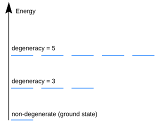
In quantum mechanics, an energy level is degenerate if it corresponds to two or more different measurable states of a quantum system. Conversely, two or more different states of a quantum mechanical system are said to be degenerate if they give the same value of energy upon measurement. The number of different states corresponding to a particular energy level is known as the degree of degeneracy of the level. It is represented mathematically by the Hamiltonian for the system having more than one linearly independent eigenstate with the same energy eigenvalue. When this is the case, energy alone is not enough to characterize what state the system is in, and other quantum numbers are needed to characterize the exact state when distinction is desired. In classical mechanics, this can be understood in terms of different possible trajectories corresponding to the same energy.
In quantum mechanics, spin is an intrinsic property of all elementary particles. All known fermions, the particles that constitute ordinary matter, have a spin of 1/2. The spin number describes how many symmetrical facets a particle has in one full rotation; a spin of 1/2 means that the particle must be rotated by two full turns before it has the same configuration as when it started.
In quantum mechanics, the angular momentum operator is one of several related operators analogous to classical angular momentum. The angular momentum operator plays a central role in the theory of atomic and molecular physics and other quantum problems involving rotational symmetry. Such an operator is applied to a mathematical representation of the physical state of a system and yields an angular momentum value if the state has a definite value for it. In both classical and quantum mechanical systems, angular momentum is one of the three fundamental properties of motion.
In quantum mechanics, Landau quantization refers to the quantization of the cyclotron orbits of charged particles in a uniform magnetic field. As a result, the charged particles can only occupy orbits with discrete, equidistant energy values, called Landau levels. These levels are degenerate, with the number of electrons per level directly proportional to the strength of the applied magnetic field. It is named after the Soviet physicist Lev Landau.
Photon polarization is the quantum mechanical description of the classical polarized sinusoidal plane electromagnetic wave. An individual photon can be described as having right or left circular polarization, or a superposition of the two. Equivalently, a photon can be described as having horizontal or vertical linear polarization, or a superposition of the two.
The theoretical and experimental justification for the Schrödinger equation motivates the discovery of the Schrödinger equation, the equation that describes the dynamics of nonrelativistic particles. The motivation uses photons, which are relativistic particles with dynamics described by Maxwell's equations, as an analogue for all types of particles.
In quantum mechanics, the Pauli equation or Schrödinger–Pauli equation is the formulation of the Schrödinger equation for spin-½ particles, which takes into account the interaction of the particle's spin with an external electromagnetic field. It is the non-relativistic limit of the Dirac equation and can be used where particles are moving at speeds much less than the speed of light, so that relativistic effects can be neglected. It was formulated by Wolfgang Pauli in 1927.
A hydrogen-like atom (or hydrogenic atom) is any atom or ion with a single valence electron. These atoms are isoelectronic with hydrogen. Examples of hydrogen-like atoms include, but are not limited to, hydrogen itself, all alkali metals such as Rb and Cs, singly ionized alkaline earth metals such as Ca+ and Sr+ and other ions such as He+, Li2+, and Be3+ and isotopes of any of the above. A hydrogen-like atom includes a positively charged core consisting of the atomic nucleus and any core electrons as well as a single valence electron. Because helium is common in the universe, the spectroscopy of singly ionized helium is important in EUV astronomy, for example, of DO white dwarf stars.
In quantum mechanics, a raising or lowering operator is an operator that increases or decreases the eigenvalue of another operator. In quantum mechanics, the raising operator is sometimes called the creation operator, and the lowering operator the annihilation operator. Well-known applications of ladder operators in quantum mechanics are in the formalisms of the quantum harmonic oscillator and angular momentum.
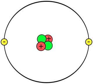
A helium atom is an atom of the chemical element helium. Helium is composed of two electrons bound by the electromagnetic force to a nucleus containing two protons along with either one or two neutrons, depending on the isotope, held together by the strong force. Unlike for hydrogen, a closed-form solution to the Schrödinger equation for the helium atom has not been found. However, various approximations, such as the Hartree–Fock method, can be used to estimate the ground state energy and wavefunction of the atom.
In linear algebra, a raising or lowering operator is an operator that increases or decreases the eigenvalue of another operator. In quantum mechanics, the raising operator is sometimes called the creation operator, and the lowering operator the annihilation operator. Well-known applications of ladder operators in quantum mechanics are in the formalisms of the quantum harmonic oscillator and angular momentum.
Symmetries in quantum mechanics describe features of spacetime and particles which are unchanged under some transformation, in the context of quantum mechanics, relativistic quantum mechanics and quantum field theory, and with applications in the mathematical formulation of the standard model and condensed matter physics. In general, symmetry in physics, invariance, and conservation laws, are fundamentally important constraints for formulating physical theories and models. In practice, they are powerful methods for solving problems and predicting what can happen. While conservation laws do not always give the answer to the problem directly, they form the correct constraints and the first steps to solving a multitude of problems.
In pure and applied mathematics, quantum mechanics and computer graphics, a tensor operator generalizes the notion of operators which are scalars and vectors. A special class of these are spherical tensor operators which apply the notion of the spherical basis and spherical harmonics. The spherical basis closely relates to the description of angular momentum in quantum mechanics and spherical harmonic functions. The coordinate-free generalization of a tensor operator is known as a representation operator.
Magnetic resonance is a quantum mechanical resonant effect that can appear when a magnetic dipole is exposed to a static magnetic field and perturbed with another, oscillating electromagnetic field. Due to the static field, the dipole can assume a number of discrete energy eigenstates, depending on the value of its angular momentum quantum number. The oscillating field can then make the dipole transit between its energy states with a certain probability and at a certain rate. The overall transition probability will depend on the field's frequency and the rate will depend on its amplitude. When the frequency of that field leads to the maximum possible transition probability between two states, a magnetic resonance has been achieved. In that case, the energy of the photons composing the oscillating field matches the energy difference between said states. If the dipole is tickled with a field oscillating far from resonance, it is unlikely to transition. That is analogous to other resonant effects, such as with the forced harmonic oscillator. The periodic transition between the different states is called Rabi cycle and the rate at which that happens is called Rabi frequency. The Rabi frequency should not be confused with the field's own frequency. Since many atomic nuclei species can behave as a magnetic dipole, this resonance technique is the basis of nuclear magnetic resonance, including nuclear magnetic resonance imaging and nuclear magnetic resonance spectroscopy.
↑ Feynman, R. P. (1985). "Electrons and their interactions". QED: The Strange Theory of Light and Matter. Princeton, New Jersey: Princeton University Press. p.115. ISBN978-0-691-08388-9. After some years, it was discovered that this value [−1/2g] was not exactly 1, but slightly more – something like 1.00116. This correction was worked out for the first time in 1948 by Schwinger as j × j divided by 2π[sic] [where j is the square root of the fine-structure constant], and was due to an alternative way the electron can go from place to place: Instead of going directly from one point to another, the electron goes along for a while and suddenly emits a photon; then (horrors!) it absorbs its own photon.
Thompson, William J. (1994). Angular Momentum: An Illustrated Guide to Rotational Symmetries for Physical Systems. Wiley. ISBN978-0-471-55264-2.
Tipler, Paul (2004). Physics for Scientists and Engineers: Mechanics, Oscillations and Waves, Thermodynamics (5thed.). W. H. Freeman. ISBN978-0-7167-0809-4.
This page is based on this Wikipedia article Text is available under the CC BY-SA 4.0 license; additional terms may apply. Images, videos and audio are available under their respective licenses.