Species distribution, or speciesdispersion,[1] is the manner in which a biological taxon is spatially arranged.[2] The geographic limits of a particular taxon's distribution is its range, often represented as shaded areas on a map. Patterns of distribution change depending on the scale at which they are viewed, from the arrangement of individuals within a small family unit, to patterns within a population, or the distribution of the entire species as a whole (range). Species distribution is not to be confused with dispersal, which is the movement of individuals away from their region of origin or from a population center of high density.
In biology, the range of a species is the geographical area within which that species can be found. Within that range, distribution is the general structure of the species population, while dispersion is the variation in its population density.
Range is often described with the following qualities:
Sometimes a distinction is made between a species' natural, endemic, indigenous, or native range, where it has historically originated and lived, and the range where a species has more recently established itself. Many terms are used to describe the new range, such as non-native, naturalized, introduced, transplanted, invasive, or colonized range.[3]Introduced typically means that a species has been transported by humans (intentionally or accidentally) across a major geographical barrier.[4]
For species found in different regions at different times of year, especially seasons, terms such as summer range and winter range are often employed.
For species for which only part of their range is used for breeding activity, the terms breeding range and non-breeding range are used.
For mobile animals, the term natural range is often used, as opposed to areas where it occurs as a vagrant.
Geographic or temporal qualifiers are often added, such as in British range or pre-1950 range. The typical geographic ranges could be the latitudinal range and elevational range.
Disjunct distribution occurs when two or more areas of the range of a taxon are considerably separated from each other geographically.
Factors affecting species distribution
Distribution patterns may change by season, distribution by humans, in response to the availability of resources, and other abiotic and biotic factors.
Abiotic
There are three main types of abiotic factors:
climatic factors consist of sunlight, atmosphere, humidity, temperature, and salinity;
edaphic factors are abiotic factors regarding soil, such as the coarseness of soil, local geology, soil pH, and aeration; and
social factors include land use and water availability.
An example of the effects of abiotic factors on species distribution can be seen in drier areas, where most individuals of a species will gather around water sources, forming a clumped distribution.
Researchers from the Arctic Ocean Diversity (ARCOD) project have documented rising numbers of warm-water crustaceans in the seas around Norway's Svalbard Islands. ARCOD is part of the Census of Marine Life, a huge 10-year project involving researchers in more than 80 nations that aims to chart the diversity, distribution and abundance of life in the oceans. Marine Life has become largely affected by increasing effects of global climate change. This study shows that as the ocean temperatures rise species are beginning to travel into the cold and harsh Arctic waters. Even the snow crab has extended its range 500km north.
Biotic
Biotic factors such as predation, disease, and inter- and intra-specific competition for resources such as food, water, and mates can also affect how a species is distributed. For example, biotic factors in a quail's environment would include their prey (insects and seeds), competition from other quail, and their predators, such as the coyote.[5] An advantage of a herd, community, or other clumped distribution allows a population to detect predators earlier, at a greater distance, and potentially mount an effective defense. Due to limited resources, populations may be evenly distributed to minimize competition,[6] as is found in forests, where competition for sunlight produces an even distribution of trees.[7]
One key factor in determining species distribution is the phenology of the organism. Plants are well documented as examples showing how phenology is an adaptive trait that can influence fitness in changing climates.[8] Physiology can influence species distributions in an environmentally sensitive manner because physiology underlies movement such as exploration and dispersal. Individuals that are more disperse-prone have higher metabolism, locomotor performance, corticosterone levels, and immunity.[9]
Humans are one of the largest distributors due to the current trends in globalization and the expanse of the transportation industry. For example, large tankers often fill their ballasts with water at one port and empty them in another, causing a wider distribution of aquatic species.[10]
Patterns on large scales
On large scales, the pattern of distribution among individuals in a population is clumped.[11]
One common example of bird species' ranges are land mass areas bordering water bodies, such as oceans, rivers, or lakes; they are called a coastal strip. A second example, some species of bird depend on water, usually a river, swamp, etc., or water related forest and live in a river corridor. A separate example of a river corridor would be a river corridor that includes the entire drainage, having the edge of the range delimited by mountains, or higher elevations; the river itself would be a smaller percentage of this entire wildlife corridor, but the corridor is created because of the river.
A further example of a bird wildlife corridor would be a mountain range corridor. In the U.S. of North America, the Sierra Nevada range in the west, and the Appalachian Mountains in the east are two examples of this habitat, used in summer, and winter, by separate species, for different reasons.
Bird species in these corridors are connected to a main range for the species (contiguous range) or are in an isolated geographic range and be a disjunct range. Birds leaving the area, if they migrate, would leave connected to the main range or have to fly over land not connected to the wildlife corridor; thus, they would be passage migrants over land that they stop on for an intermittent, hit or miss, visit.
Patterns on small scales
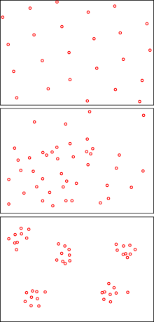
Three basic types of population distribution within a regional range are (from top to bottom) uniform, random, and clumped.
On large scales, the pattern of distribution among individuals in a population is clumped. On small scales, the pattern may be clumped, regular, or random.[11]
Clumped
Clumped distribution, also called aggregated distribution, clumped dispersion or patchiness, is the most common type of dispersion found in nature. In clumped distribution, the distance between neighboring individuals is minimized. This type of distribution is found in environments that are characterized by patchy resources. Animals need certain resources to survive, and when these resources become rare during certain parts of the year animals tend to "clump" together around these crucial resources. Individuals might be clustered together in an area due to social factors such as selfish herds and family groups. Organisms that usually serve as prey form clumped distributions in areas where they can hide and detect predators easily.
Other causes of clumped distributions are the inability of offspring to independently move from their habitat. This is seen in juvenile animals that are immobile and strongly dependent upon parental care. For example, the bald eagle's nest of eaglets exhibits a clumped species distribution because all the offspring are in a small subset of a survey area before they learn to fly. Clumped distribution can be beneficial to the individuals in that group. However, in some herbivore cases, such as cows and wildebeests, the vegetation around them can suffer, especially if animals target one plant in particular.
Clumped distribution in species acts as a mechanism against predation as well as an efficient mechanism to trap or corner prey. African wild dogs, Lycaon pictus, use the technique of communal hunting to increase their success rate at catching prey. Studies have shown that larger packs of African wild dogs tend to have a greater number of successful kills. A prime example of clumped distribution due to patchy resources is the wildlife in Africa during the dry season; lions, hyenas, giraffes, elephants, gazelles, and many more animals are clumped by small water sources that are present in the severe dry season.[12] It has also been observed that extinct and threatened species are more likely to be clumped in their distribution on a phylogeny. The reasoning behind this is that they share traits that increase vulnerability to extinction because related taxa are often located within the same broad geographical or habitat types where human-induced threats are concentrated. Using recently developed complete phylogenies for mammalian carnivores and primates it has been shown that in the majority of instances threatened species are far from randomly distributed among taxa and phylogeneticclades and display clumped distribution.[13]
A contiguous distribution is one in which individuals are closer together than they would be if they were randomly or evenly distributed, i.e., it is clumped distribution with a single clump.[14]
Regular or uniform
Less common than clumped distribution, uniform distribution, also known as even distribution, is evenly spaced.[15] Uniform distributions are found in populations in which the distance between neighboring individuals is maximized. The need to maximize the space between individuals generally arises from competition for a resource such as moisture or nutrients, or as a result of direct social interactions between individuals within the population, such as territoriality. For example, penguins often exhibit uniform spacing by aggressively defending their territory among their neighbors. The burrows of great gerbils for example are also regularly distributed,[16] which can be seen on satellite images.[17] Plants also exhibit uniform distributions, like the creosote bushes in the southwestern region of the United States. Salvia leucophylla is a species in California that naturally grows in uniform spacing. This flower releases chemicals called terpenes which inhibit the growth of other plants around it and results in uniform distribution.[18] This is an example of allelopathy, which is the release of chemicals from plant parts by leaching, root exudation, volatilization, residue decomposition and other processes. Allelopathy can have beneficial, harmful, or neutral effects on surrounding organisms. Some allelochemicals even have selective effects on surrounding organisms; for example, the tree species Leucaena leucocephala exudes a chemical that inhibits the growth of other plants but not those of its own species, and thus can affect the distribution of specific rival species. Allelopathy usually results in uniform distributions, and its potential to suppress weeds is being researched.[19] Farming and agricultural practices often create uniform distribution in areas where it would not previously exist, for example, orange trees growing in rows on a plantation.
Random
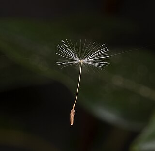
Random distribution, also known as unpredictable spacing, is the least common form of distribution in nature and occurs when the members of a given species are found in environments in which the position of each individual is independent of the other individuals: they neither attract nor repel one another. Random distribution is rare in nature as biotic factors, such as the interactions with neighboring individuals, and abiotic factors, such as climate or soil conditions, generally cause organisms to be either clustered or spread. Random distribution usually occurs in habitats where environmental conditions and resources are consistent. This pattern of dispersion is characterized by the lack of any strong social interactions between species. For example; When dandelionseeds are dispersed by wind, random distribution will often occur as the seedlings land in random places determined by uncontrollable factors. Oyster larvae can also travel hundreds of kilometers powered by sea currents, which can result in their random distribution. Random distributions exhibit chance clumps (see Poisson clumping).
Statistical determination of distribution patterns
There are various ways to determine the distribution pattern of species. The Clark–Evans nearest neighbor method[20] can be used to determine if a distribution is clumped, uniform, or random.[21] To utilize the Clark–Evans nearest neighbor method, researchers examine a population of a single species. The distance of an individual to its nearest neighbor is recorded for each individual in the sample. For two individuals that are each other's nearest neighbor, the distance is recorded twice, once for each individual. To receive accurate results, it is suggested that the number of distance measurements is at least 50. The average distance between nearest neighbors is compared to the expected distance in the case of random distribution to give the ratio:
If this ratio R is equal to 1, then the population is randomly dispersed. If R is significantly greater than1, the population is evenly dispersed. Lastly, if R is significantly less than1, the population is clumped. Statistical tests (such as t-test, chi squared, etc.) can then be used to determine whether R is significantly different from1.
The variance/mean ratio method focuses mainly on determining whether a species fits a randomly spaced distribution, but can also be used as evidence for either an even or clumped distribution.[22] To utilize the Variance/Mean ratio method, data is collected from several random samples of a given population. In this analysis, it is imperative that data from at least 50 sample plots is considered. The number of individuals present in each sample is compared to the expected counts in the case of random distribution. The expected distribution can be found using Poisson distribution. If the variance/mean ratio is equal to 1, the population is found to be randomly distributed. If it is significantly greater than 1, the population is found to be clumped distribution. Finally, if the ratio is significantly less than 1, the population is found to be evenly distributed. Typical statistical tests used to find the significance of the variance/mean ratio include Student's t-test and chi squared.
However, many researchers believe that species distribution models based on statistical analysis, without including ecological models and theories, are too incomplete for prediction. Instead of conclusions based on presence-absence data, probabilities that convey the likelihood a species will occupy a given area are more preferred because these models include an estimate of confidence in the likelihood of the species being present/absent. They are also more valuable than data collected based on simple presence or absence because models based on probability allow the formation of spatial maps that indicates how likely a species is to be found in a particular area. Similar areas can then be compared to see how likely it is that a species will occur there also; this leads to a relationship between habitat suitability and species occurrence.[23]
Species distribution can be predicted based on the pattern of biodiversity at spatial scales. A general hierarchical model can integrate disturbance, dispersal and population dynamics. Based on factors of dispersal, disturbance, resources limiting climate, and other species distribution, predictions of species distribution can create a bio-climate range, or bio-climate envelope. The envelope can range from a local to a global scale or from a density independence to dependence. The hierarchical model takes into consideration the requirements, impacts or resources as well as local extinctions in disturbance factors. Models can integrate the dispersal/migration model, the disturbance model, and abundance model. Species distribution models (SDMs) can be used to assess climate change impacts and conservation management issues. Species distribution models include: presence/absence models, the dispersal/migration models, disturbance models, and abundance models. A prevalent way of creating predicted distribution maps for different species is to reclassify a land cover layer depending on whether or not the species in question would be predicted to habit each cover type. This simple SDM is often modified through the use of range data or ancillary information, such as elevation or water distance.
Recent studies have indicated that the grid size used can have an effect on the output of these species distribution models.[24] The standard 50x50 km grid size can select up to 2.89 times more area than when modeled with a 1x1 km grid for the same species. This has several effects on the species conservation planning under climate change predictions (global climate models, which are frequently used in the creation of species distribution models, usually consist of 50–100km size grids) which could lead to over-prediction of future ranges in species distribution modeling. This can result in the misidentification of protected areas intended for a species future habitat.
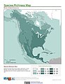
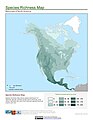
Species Distribution Grids Project
The Species Distribution Grids Project is an effort led out of the University of Columbia to create maps and databases of the whereabouts of various animal species. This work is centered on preventing deforestation and prioritizing areas based on species richness.[25] As of April 2009, data are available for global amphibian distributions, as well as birds and mammals in the Americas. The map gallery Gridded Species Distribution contains sample maps for the Species Grids data set. These maps are not inclusive but rather contain a representative sample of the types of data available for download:
↑ Hülsmann, Norbert; Galil, Bella S. (2002), Leppäkoski, Erkki; Gollasch, Stephan; Olenin, Sergej (eds.), "Protists — A Dominant Component of the Ballast-Transported Biota", Invasive Aquatic Species of Europe. Distribution, Impacts and Management, Springer Netherlands, pp.20–26, doi:10.1007/978-94-015-9956-6_3, ISBN9789401599566
↑ Philip J. Clark and Francis C. Evans (Oct 1954). "Distance to Nearest Neighbor as a Measure of Spatial Relationships in Populations". Ecology. 35 (4). Ecological Society of America: 445–453. Bibcode:1954Ecol...35..445C. doi:10.2307/1931034. JSTOR1931034.
↑ Blackith, R. E. (1958). Nearest-Neighbour Distance Measurements for the Estimation of Animal Populations. Ecology. pp.147–150.
↑ Banerjee, B. (1976). Variance to mean ratio and the spatial distribution of animals. Birkhäuser Basel. pp.993–994.
In ecology, a niche is the match of a species to a specific environmental condition. It describes how an organism or population responds to the distribution of resources and competitors and how it in turn alters those same factors. "The type and number of variables comprising the dimensions of an environmental niche vary from one species to another [and] the relative importance of particular environmental variables for a species may vary according to the geographic and biotic contexts".
Biogeography is the study of the distribution of species and ecosystems in geographic space and through geological time. Organisms and biological communities often vary in a regular fashion along geographic gradients of latitude, elevation, isolation and habitat area. Phytogeography is the branch of biogeography that studies the distribution of plants. Zoogeography is the branch that studies distribution of animals. Mycogeography is the branch that studies distribution of fungi, such as mushrooms.
This glossary of ecology is a list of definitions of terms and concepts in ecology and related fields. For more specific definitions from other glossaries related to ecology, see Glossary of biology, Glossary of evolutionary biology, and Glossary of environmental science.
Biological dispersal refers to both the movement of individuals from their birth site to their breeding site and the movement from one breeding site to another . Dispersal is also used to describe the movement of propagules such as seeds and spores. Technically, dispersal is defined as any movement that has the potential to lead to gene flow. The act of dispersal involves three phases: departure, transfer, and settlement. There are different fitness costs and benefits associated with each of these phases. Through simply moving from one habitat patch to another, the dispersal of an individual has consequences not only for individual fitness, but also for population dynamics, population genetics, and species distribution. Understanding dispersal and the consequences, both for evolutionary strategies at a species level and for processes at an ecosystem level, requires understanding on the type of dispersal, the dispersal range of a given species, and the dispersal mechanisms involved. Biological dispersal can be correlated to population density. The range of variations of a species' location determines the expansion range.
Spatial ecology studies the ultimate distributional or spatial unit occupied by a species. In a particular habitat shared by several species, each of the species is usually confined to its own microhabitat or spatial niche because two species in the same general territory cannot usually occupy the same ecological niche for any significant length of time.
Colonisation or colonization is the spread and development of an organism in a new area or habitat. Colonization comprises the physical arrival of a species in a new area, but also its successful establishment within the local community. In ecology, it is represented by the symbol λ to denote the long-term intrinsic growth rate of a population.
In marine environments, a nursery habitat is a subset of all habitats where juveniles of a species occur, having a greater level of productivity per unit area than other juvenile habitats. Mangroves, salt marshes and seagrass are typical nursery habitats for a range of marine species. Some species will use nonvegetated sites, such as the yellow-eyed mullet, blue sprat and flounder.
In landscape ecology, landscape connectivity is, broadly, "the degree to which the landscape facilitates or impedes movement among resource patches". Alternatively, connectivity may be a continuous property of the landscape and independent of patches and paths. Connectivity includes both structural connectivity and functional connectivity. Functional connectivity includes actual connectivity and potential connectivity in which movement paths are estimated using the life-history data.
In ecology, an ideal free distribution (IFD) is a theoretical way in which a population's individuals distribute themselves among several patches of resources within their environment, in order to minimize resource competition and maximize fitness. The theory states that the number of individual animals that will aggregate in various patches is proportional to the amount of resources available in each. For example, if patch A contains twice as many resources as patch B, there will be twice as many individuals foraging in patch A as in patch B.
Spatial descriptive statistics is the intersection of spatial statistics and descriptive statistics; these methods are used for a variety of purposes in geography, particularly in quantitative data analyses involving Geographic Information Systems (GIS).
The following outline is provided as an overview of and topical guide to ecology:
In ecology, the occupancy–abundance (O–A) relationship is the relationship between the abundance of species and the size of their ranges within a region. This relationship is perhaps one of the most well-documented relationships in macroecology, and applies both intra- and interspecifically. In most cases, the O–A relationship is a positive relationship. Although an O–A relationship would be expected, given that a species colonizing a region must pass through the origin and could reach some theoretical maximum abundance and distribution, the relationship described here is somewhat more substantial, in that observed changes in range are associated with greater-than-proportional changes in abundance. Although this relationship appears to be pervasive, and has important implications for the conservation of endangered species, the mechanism(s) underlying it remain poorly understood.
In probability theory and statistics, the index of dispersion, dispersion index, coefficient of dispersion, relative variance, or variance-to-mean ratio (VMR), like the coefficient of variation, is a normalized measure of the dispersion of a probability distribution: it is a measure used to quantify whether a set of observed occurrences are clustered or dispersed compared to a standard statistical model.
Spatial organization can be observed when components of an abiotic or biological group are arranged non-randomly in space. Abiotic patterns, such as the ripple formations in sand dunes or the oscillating wave patterns of the Belousov–Zhabotinsky reaction emerge after thousands of particles interact millions of times. On the other hand, individuals in biological groups may be arranged non-randomly due to selfish behavior, dominance interactions, or cooperative behavior. W. D. Hamilton (1971) proposed that in a non-related "herd" of animals, the spatial organization is likely a result of the selfish interests of individuals trying to acquire food or avoid predation. On the other hand, spatial arrangements have also been observed among highly related members of eusocial groups, suggesting that the arrangement of individuals may provide advantages for the group.
The body size-species richness distribution is a pattern observed in the way taxa are distributed over large spatial scales. The number of species that exhibit small body size generally far exceed the number of species that are large-bodied. Macroecology has long sought to understand the mechanisms that underlie the patterns of biodiversity, such as the body size-species richness pattern.
Isolation by distance (IBD) is a term used to refer to the accrual of local genetic variation under geographically limited dispersal. The IBD model is useful for determining the distribution of gene frequencies over a geographic region. Both dispersal variance and migration probabilities are variables in this model and both contribute to local genetic differentiation. Isolation by distance is usually the simplest model for the cause of genetic isolation between populations. Evolutionary biologists and population geneticists have been exploring varying theories and models for explaining population structure. Yoichi Ishida compares two important theories of isolation by distance and clarifies the relationship between the two. According to Ishida, Sewall Wright's isolation by distance theory is termed ecological isolation by distance while Gustave Malécot's theory is called genetic isolation by distance. Isolation by distance is distantly related to speciation. Multiple types of isolating barriers, namely prezygotic isolating barriers, including isolation by distance, are considered the key factor in keeping populations apart, limiting gene flow.
Species distribution modelling (SDM), also known as environmental(or ecological) niche modelling (ENM), habitat modelling, predictive habitat distribution modelling, and range mapping uses ecological models to predict the distribution of a species across geographic space and time using environmental data. The environmental data are most often climate data (e.g. temperature, precipitation), but can include other variables such as soil type, water depth, and land cover. SDMs are used in several research areas in conservation biology, ecology and evolution. These models can be used to understand how environmental conditions influence the occurrence or abundance of a species, and for predictive purposes (ecological forecasting). Predictions from an SDM may be of a species’ future distribution under climate change, a species’ past distribution in order to assess evolutionary relationships, or the potential future distribution of an invasive species. Predictions of current and/or future habitat suitability can be useful for management applications (e.g. reintroduction or translocation of vulnerable species, reserve placement in anticipation of climate change).
Taylor's power law is an empirical law in ecology that relates the variance of the number of individuals of a species per unit area of habitat to the corresponding mean by a power law relationship. It is named after the ecologist who first proposed it in 1961, Lionel Roy Taylor (1924–2007). Taylor's original name for this relationship was the law of the mean. The name Taylor's law was coined by Southwood in 1966.
The geographical limits to the distribution of a species are determined by biotic or abiotic factors. Core populations are those occurring within the centre of the range, and marginal populations are found at the boundary of the range.
Alien species, or species that are not native, invade habitats and alter ecosystems around the world. Invasive species are only considered invasive if they are able to survive and sustain themselves in their new environment. A habitat and the environment around it has natural flaws that make them vulnerable to invasive species. The level of vulnerability of a habitat to invasions from outside species is defined as its invasibility. One must be careful not to get this confused with invasiveness, which relates to the species itself and its ability to invade an ecosystem.
This page is based on this Wikipedia article Text is available under the CC BY-SA 4.0 license; additional terms may apply. Images, videos and audio are available under their respective licenses.