Metapopulation

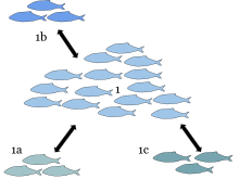
Metapopulations are important in fisheries. The local population (1.) serves as a source for hybridization with surrounding subspecies populations (1.a, 1.b, and 1.c).The populations are normally spatially separated and independent but spatial overlap between them during breeding times allows for gene flow between the populations.

A metapopulation consists of a group of spatially separated populations of the same species which interact at some level. The term metapopulation was coined by Richard Levins in 1969 to describe a model of population dynamics of insect pests in agricultural fields, but the idea has been most broadly applied to species in naturally or artificially fragmented habitats. In Levins' own words, it consists of "a population of populations". ^[1]

A metapopulation is generally considered to consist of several distinct populations together with areas of suitable habitat which are currently unoccupied. In classical metapopulation theory, each population cycles in relative independence of the other populations and eventually goes extinct as a consequence of demographic stochasticity (fluctuations in population size due to random demographic events); the smaller the population, the more chances of inbreeding depression and prone to extinction.

Although individual populations have finite life-spans, the metapopulation as a whole is often stable because immigrants from one population (which may, for example, be experiencing a population boom) are likely to re-colonize habitat which has been left open by the extinction of another population. They may also emigrate to a small population and rescue that population from extinction (called the rescue effect). Such a rescue effect may occur because declining populations leave niche opportunities open to the "rescuers".

The development of metapopulation theory, in conjunction with the development of source–sink dynamics, emphasised the importance of connectivity between seemingly isolated populations. Although no single population may be able to guarantee the long-term survival of a given species, the combined effect of many populations may be able to do this.

Metapopulation theory was first developed for terrestrial ecosystems, and subsequently applied to the marine realm. ^[2] In fisheries science, the term "sub-population" is equivalent to the metapopulation science term "local population". Most marine examples are provided by relatively sedentary species occupying discrete patches of habitat, with both local recruitment and recruitment from other local populations in the larger metapopulation. Kritzer & Sale have argued against strict application of the metapopulation definitional criteria that extinction risks to local populations must be non-negligible. ^{[2] : 32}

Finnish biologist Ilkka Hanski of the University of Helsinki was an important contributor to metapopulation theory.

Predation and oscillations

The first experiments with predation and spatial heterogeneity were conducted by G. F. Gause in the 1930s, based on the Lotka–Volterra equation, which was formulated in the mid-1920s, but no further application had been conducted. ^[3] The Lotka-Volterra equation suggested that the relationship between predators and their prey would result in population oscillations over time based on the initial densities of predator and prey. Gause's early experiments to prove the predicted oscillations of this theory failed because the predator–prey interactions were not influenced by immigration. However, once immigration was introduced, the population cycles accurately depicted the oscillations predicted by the Lotka-Volterra equation, with the peaks in prey abundance shifted slightly to the left of the peaks of the predator densities. Huffaker's experiments expanded on those of Gause by examining how both the factors of migration and spatial heterogeneity lead to predator–prey oscillations.

Huffaker's experiments on predator–prey interactions (1958)

In order to study predation and population oscillations, Huffaker used mite species, one being the predator and the other being the prey. ^[4] He set up a controlled experiment using oranges, which the prey fed on, as the spatially structured habitat in which the predator and prey would interact. ^[5] At first, Huffaker experienced difficulties similar to those of Gause in creating a stable predator–prey interaction. By using oranges only, the prey species quickly became extinct followed consequently with predator extinction. However, he discovered that by modifying the spatial structure of the habitat, he could manipulate the population dynamics and allow the overall survival rate for both species to increase. He did this by altering the distance between the prey and oranges (their food), establishing barriers to predator movement, and creating corridors for the prey to disperse. ^[3] These changes resulted in increased habitat patches and in turn provided more areas for the prey to seek temporary protection. When the prey would become extinct locally at one habitat patch, they were able to reestablish by migrating to new patches before being attacked by predators. This habitat spatial structure of patches allowed for coexistence between the predator and prey species and promoted a stable population oscillation model. ^[6] Although the term metapopulation had not yet been coined, the environmental factors of spatial heterogeneity and habitat patchiness would later describe the conditions of a metapopulation relating to how groups of spatially separated populations of species interact with one another. Huffaker's experiment is significant because it showed how metapopulations can directly affect the predator–prey interactions and in turn influence population dynamics. ^[7]

The Levins model

Levins' original model applied to a metapopulation distributed over many patches of suitable habitat with significantly less interaction between patches than within a patch. Population dynamics within a patch were simplified to the point where only presence and absence were considered. Each patch in his model is either populated or not.

Let N be the fraction of patches occupied at a given time. During a time dt, each occupied patch can become unoccupied with an extinction probability edt. Additionally, 1 − N of the patches are unoccupied. Assuming a constant rate c of propagule generation from each of the N occupied patches, during a time dt, each unoccupied patch can become occupied with a colonization probability cNdt . Accordingly, the time rate of change of occupied patches, dN/dt, is

${\displaystyle {\frac {dN}{dt}}=cN(1-N)-eN.\,}$

This equation is mathematically equivalent to the logistic model, with a carrying capacity K given by

${\displaystyle K=1-{\frac {e}{c}}\,}$

and growth rate r

${\displaystyle r=c-e.\,}$

At equilibrium, therefore, some fraction of the species's habitat will always be unoccupied.

Stochasticity and metapopulations

Huffaker's ^[4] studies of spatial structure and species interactions are an example of early experimentation in metapopulation dynamics. Since the experiments of Huffaker ^[4] and Levins, ^[1] models have been created which integrate stochastic factors. These models have shown that the combination of environmental variability (stochasticity) and relatively small migration rates cause indefinite or unpredictable persistence. However, Huffaker's experiment almost guaranteed infinite persistence because of the controlled immigration variable.

Stochastic patch occupancy models (SPOMs)

One major drawback of the Levins model is that it is deterministic, whereas the fundamental metapopulation processes are stochastic. Metapopulations are particularly useful when discussing species in disturbed habitats, and the viability of their populations, i.e., how likely they are to become extinct in a given time interval. The Levins model cannot address this issue. A simple way to extend the Levins' model to incorporate space and stochastic considerations is by using the contact process. Simple modifications to this model can also incorporate for patch dynamics. At a given percolation threshold, habitat fragmentation effects take place in these configurations predicting more drastic extinction thresholds. ^[8]

For conservation biology purposes, metapopulation models must include (a) the finite nature of metapopulations (how many patches are suitable for habitat), and (b) the probabilistic nature of extinction and colonisation. Also, note that in order to apply these models, the extinctions and colonisations of the patches must be asynchronous.

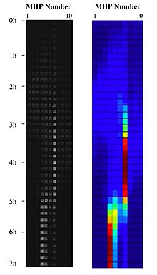
Microhabitat patches (MHPs) and bacterial metapopulations

E. coli metapopulation on a chip.

Combining nanotechnology with landscape ecology, synthetic habitat landscapes have been fabricated on a chip by building a collection of bacterial mini-habitats with nano-scale channels providing them with nutrients for habitat renewal, and connecting them by corridors in different topological arrangements, generating a spatial mosaic of patches of opportunity distributed in time. This can be used for landscape experiments by studying the bacteria metapopulations on the chip, for example their evolutionary ecology. ^[9]

Life history evolution

Metapopulation models have been used to explain life-history evolution, such as the ecological stability of amphibian metamorphosis in small vernal ponds. Alternative ecological strategies have evolved. For example, some salamanders forgo metamorphosis and sexually mature as aquatic neotenes. The seasonal duration of wetlands and the migratory range of the species determines which ponds are connected and if they form a metapopulation. The duration of the life history stages of amphibians relative to the duration of the vernal pool before it dries up regulates the ecological development of metapopulations connecting aquatic patches to terrestrial patches. ^[10]

See also

• Competition (biology)
• Conservation biology
• Landscape ecology
• Lotka–Volterra equations
• Oscillation
• Population viability analysis
• Predation
• Spatial heterogeneity

References

1. Levins, R. (1969), "Some demographic and genetic consequences of environmental heterogeneity for biological control", Bulletin of the Entomological Society of America, 15 (3): 237–240, doi:10.1093/besa/15.3.237
2. Kritzer, J. P. & Sale, P. F. (eds) (2006) Marine metapopulations, Academic Press, New York.
3. Real, Leslie A. and Brown, James H. 1991. Foundations of Ecology: Classic papers with commentaries. The University of Chicago Press, Chicago.
4. Huffaker, C.B. (1958), "Experimental Studies on Predation: Dispersion factors and predator–prey oscillations", Hilgardia, 27 (343): 343–383, doi: 10.3733/hilg.v27n14p343
5. Legendre, P.; Fortin, M.J. (1989), "Spatial pattern and ecological analysis", Plant Ecology, 80 (2): 107, CiteSeerX   10.1.1.330.8940 , doi:10.1007/BF00048036, S2CID   17101938
6. Kareiva, P. (1987), "Habitat Fragmentation and the Stability of Predator–Prey Interactions", Nature, 326 (6111): 388–390, Bibcode:1987Natur.326..388K, doi:10.1038/326388a0, S2CID   4335135
7. Janssen, A. et al. 1997. Metapopulation Dynamics of a Persisting Predator–Prey system.
8. Keymer J.E; P.A. Marquet; J.X. Velasco‐Hernández; S.A. Levin (November 2000). "Extinction Thresholds and Metapopulation Persistence in Dynamic Landscapes". The American Naturalist. 156 (5): 478–4945. doi:10.1086/303407. hdl: 10533/172124 . PMID   29587508. S2CID   4385886.
9. Keymer J.E.; P. Galajda; C. Muldoon R. & R. Austin (November 2006). "Bacterial metapopulations in nanofabricated landscapes". PNAS. 103 (46): 17290–295. Bibcode:2006PNAS..10317290K. doi: 10.1073/pnas.0607971103 . PMC   1635019 . PMID   17090676.
10. Petranka, J. W. (2007), "Evolution of complex life cycles of amphibians: bridging the gap between metapopulation dynamics and life history evolution", Evolutionary Ecology, 21 (6): 751–764, doi:10.1007/s10682-006-9149-1, S2CID   38832436.

• Bascompte J.; Solé R. V. (1996), "Habitat Fragmentation and Extinction Thresholds in spatially explicit models", Journal of Animal Ecology, 65 (4): 465–473, doi:10.2307/5781, JSTOR   5781.
• Hanski, I. Metapopulation Ecology Oxford University Press. 1999. ISBN   0-19-854065-5
• Fahrig, L. 2003. Effects of Habitat Fragmentation on Biodiversity. Annual Review of ecology, evolution, and systematics. 34:1, p. 487.
• Levin S.A. (1974), "Dispersion and Population Interactions", The American Naturalist, 108 (960): 207, doi:10.1086/282900, S2CID   83630608.

External links

• Helsinki-science: Metapopulation