Geophysical fluid dynamics

Model forecast of Hurricane Mitch created by the Geophysical Fluid Dynamics Laboratory. The arrows are wind vectors and the grey shading indicates an equivalent potential temperature surface that highlights the surface inflow layer and eyewall region.

Geophysical fluid dynamics, in its broadest meaning, refers to the fluid dynamics of naturally occurring flows, such as lava flows, oceans, and planetary atmospheres, on Earth and other planets. ^[1]

Two physical features that are common to many of the phenomena studied in geophysical fluid dynamics are rotation of the fluid due to the planetary rotation and stratification (layering). The applications of geophysical fluid dynamics do not generally include the circulation of the mantle, which is the subject of geodynamics, or fluid phenomena in the magnetosphere.

Fundamentals

To describe the flow of geophysical fluids, equations are needed for conservation of momentum (or Newton's second law) and conservation of energy. The former leads to the Navier–Stokes equations which cannot be solved analytically (yet). Therefore, further approximations are generally made in order to be able to solve these equations. First, the fluid is assumed to be incompressible. Remarkably, this works well even for a highly compressible fluid like air as long as sound and shock waves can be ignored. ^{[2] : 2–3} Second, the fluid is assumed to be a Newtonian fluid, meaning that there is a linear relation between the shear stress τ and the strain u, for example

${\displaystyle \tau =\mu {\frac {du}{dx}},}$

where μ is the viscosity. ^{[2] : 2–3} Under these assumptions the Navier-Stokes equations are

${\displaystyle \overbrace {\rho {\Big (}\underbrace {\frac {\partial \mathbf {v} }{\partial t}} _{\begin{smallmatrix}{\text{Eulerian}}\\{\text{acceleration}}\end{smallmatrix}}+\underbrace {\mathbf {v} \cdot \nabla \mathbf {v} } _{\begin{smallmatrix}{\text{Advection}}\end{smallmatrix}}{\Big )}} ^{\text{Inertia (per volume)}}=\overbrace {\underbrace {-\nabla p} _{\begin{smallmatrix}{\text{Pressure}}\\{\text{gradient}}\end{smallmatrix}}+\underbrace {\mu \nabla ^{2}\mathbf {v} } _{\text{Viscosity}}} ^{\text{Divergence of stress}}+\underbrace {\mathbf {f} } _{\begin{smallmatrix}{\text{Other}}\\{\text{body}}\\{\text{forces}}\end{smallmatrix}}.}$

The left hand side represents the acceleration that a small parcel of fluid would experience in a reference frame that moved with the parcel (a Lagrangian frame of reference). In a stationary (Eulerian) frame of reference, this acceleration is divided into the local rate of change of velocity and advection, a measure of the rate of flow in or out of a small region. ^{[2] : 44–45}

The equation for energy conservation is essentially an equation for heat flow. If heat is transported by conduction, the heat flow is governed by a diffusion equation. If there are also buoyancy effects, for example hot air rising, then natural convection, also known as free convection, can occur. ^{[2] : 171} Convection in the Earth's outer core drives the geodynamo that is the source of the Earth's magnetic field. ^{[3] : Chapter 8} In the ocean, convection can be thermal (driven by heat), haline (where the buoyancy is due to differences in salinity), or thermohaline , a combination of the two. ^[4]

Buoyancy and stratification

Internal waves in the Strait of Messina (photographed by ASTER).

Fluid that is less dense than its surroundings tends to rise until it has the same density as its surroundings. If there is not much energy input to the system, it will tend to become stratified. On a large scale, Earth's atmosphere is divided into a series of layers. Going upwards from the ground, these are the troposphere, stratosphere, mesosphere, thermosphere, and exosphere. ^[5]

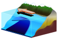
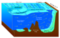
The density of air is mainly determined by temperature and water vapor content, the density of sea water by temperature and salinity, and the density of lake water by temperature. Where stratification occurs, there may be thin layers in which temperature or some other property changes more rapidly with height or depth than the surrounding fluid. Depending on the main sources of buoyancy, this layer may be called a pycnocline (density), thermocline (temperature), halocline (salinity), or chemocline (chemistry, including oxygenation).

The same buoyancy that gives rise to stratification also drives gravity waves. If the gravity waves occur within the fluid, they are called internal waves. ^{[2] : 208–214}

In modeling buoyancy-driven flows, the Navier-Stokes equations are modified using the Boussinesq approximation. This ignores variations in density except where they are multiplied by the gravitational acceleration g. ^{[2] : 188}

If the pressure depends only on density and vice versa, the fluid dynamics are called barotropic. In the atmosphere, this corresponds to a lack of fronts, as in the tropics. If there are fronts, the flow is baroclinic, and instabilities such as cyclones can occur. ^[6]

Rotation

• Coriolis effect
• Circulation
• Kelvin's circulation theorem
• Vorticity equation
• Thermal wind
• Geostrophic current
• Geostrophic wind
• Taylor–Proudman theorem
• Hydrostatic equilibrium
• Ekman spiral
• Ekman layer

General circulation

• Atmospheric circulation
• Ocean current
• Ocean dynamics
• Thermohaline circulation
• Boundary current
• Sverdrup balance
• Subsurface currents

Waves

Barotropic

• Kelvin wave
• Rossby wave
• Sverdrup wave (Poincaré wave)

Baroclinic

• Gravity wave

See also

• Geophysical Fluid Dynamics Laboratory

References

1. Vallis, Geoffrey K. (24 August 2016). "Geophysical fluid dynamics: whence, whither and why?". Proceedings of the Royal Society A: Mathematical, Physical and Engineering Sciences. 472 (2192): 20160140. Bibcode:2016RSPSA.47260140V. doi:10.1098/rspa.2016.0140. PMC   5014103 . PMID   27616918.
2. Tritton, D. J. (1990). Physical Fluid Dynamics (Second ed.). Oxford University Press. ISBN   0-19-854489-8.
3. Merrill, Ronald T.; McElhinny, Michael W.; McFadden, Phillip L. (1996). The magnetic field of the earth: paleomagnetism, the core, and the deep mantle. Academic Press. ISBN   978-0-12-491246-5.
4. Soloviev, A.; Klinger, B. (2009). "Open ocean circulation". In Thorpe, Steve A. (ed.). Encyclopedia of ocean sciences elements of physical oceanography. London: Academic Press. p. 414. ISBN   9780123757210.
5. Zell, Holly (2015-03-02). "Earth's Upper Atmosphere". NASA. Retrieved 2017-02-20.
6. Haby, Jeff. "Barotropic and baroclinic defined". Haby's weather forecasting hints. Retrieved 17 August 2017.

Further reading

• Cushman-Roisin, Benoit; Beckers, Jean-Marie (October 2011). Introduction to Geophysical Fluid Dynamics: Physical and Numerical Aspects (Second ed.). Academic Press. ISBN   978-0-12-088759-0 . Retrieved October 14, 2010.
• Gill, Adrian E. (1982). Atmosphere : Ocean dynamics ([Nachdr.] ed.). New York: Academic Press. ISBN   978-0122835223.
• McWilliams, James C. (2006). Fundamentals of geophysical fluid dynamics. Cambridge: Cambridge Univ. Press. ISBN   9780521856379.
• Monin, A.S. (1990). Theoretical Geophysical Fluid Dynamics. Dordrecht: Springer Netherlands. ISBN   978-94-009-1880-1.
• Pedlosky, Joseph (2012). Geophysical Fluid Dynamics. Springer Science & Business Media. ISBN   9781468400717.
• Salmon, Rick (1998). Lectures on Geophysical Fluid Dynamics. Oxford University Press. ISBN   9780195355321.
• Vallis, Geoffrey K. (2006). Atmospheric and oceanic fluid dynamics : fundamentals and large-scale circulation (Reprint ed.). Cambridge: Cambridge University Press. ISBN   978-0521849692.

External links

• Geophysical Fluid Dynamics Program (Woods Hole Oceanographic Institution)
• Geophysical Fluid Dynamics Laboratory (University of Washington)