The Phillips curve is a representation of the relationship between unemployment and inflation in the macroeconomy, where a tradeoff between low unemployment and price stability exists.[1] Identified by economist Bill Phillips, the curve shows a relationship between lowering unemployment with increasing wages in an economy.[2] While Phillips did not directly link employment and inflation, this was a trivial deduction from his statistical findings. Classical economists Paul Samuelson and Robert Solow made the connection explicit, followed by the theoretical arguments developed by Milton Friedman[3] and Edmund Phelps.[4][5]
While there is a short-run tradeoff between unemployment and inflation, it has not been observed in the long run.[6] In 1967 and 1968, Friedman and Phelps asserted that the Phillips curve was only applicable in the short run and that, in the long run, inflationary policies would not decrease unemployment.[3][4][5][7] Friedman correctly predicted the stagflation of the 1970s.[8]
In the 2010s[9] the slope of the Phillips curve appears to have declined and there has been controversy over the usefulness of the Phillips curve in predicting inflation. A 2022 study found that the slope of the Phillips curve is small and was small even during the early 1980s.[10] Nonetheless, the Phillips curve is still used by central banks in understanding and forecasting inflation.[11]
History
Bill Phillips, a New Zealand born economist, wrote a paper in 1958 titled "The Relation between Unemployment and the Rate of Change of Money Wage Rates in the United Kingdom, 1861–1957", which was published in the quarterly journal Economica.[12] In the paper Phillips describes how he observed an inverse relationship between money wage changes and unemployment in the British economy over the period examined. When the demand for labour is high, and there are very few unemployed, we should expect workers to bid up wages quite rapidly, each firm and each industry being continually tempted to offer a little above the prevailing wage rates to attract the most suitable labour from other firms and industries.[12]
Similar patterns were found in other countries and in 1960 Paul Samuelson and Robert Solow took Phillips's work and made explicit the link between inflation and unemployment: when inflation was high, unemployment was low, and vice versa.[13]
In the 1920s, an American economist Irving Fisher had noted this relationship between unemployment and prices. However, Phillips's original curve described the behavior of money wages.[14]
In the years following Phillips's 1958 paper, many economists in advanced industrial countries believed that his results showed a permanently stable relationship between inflation and unemployment.[citation needed] One implication of this was that governments could control unemployment and inflation with a Keynesian policy. They could tolerate a reasonably high inflation as this would lead to lower unemployment – there would be a trade-off between inflation and unemployment. For example, monetary policy and/or fiscal policy could be used to stimulate the economy, raising gross domestic product and lowering the unemployment rate. Moving along the Phillips curve, this would lead to a higher inflation rate, the cost of enjoying lower unemployment rates.[citation needed] Economist James Forder disputes this history and argues that it is a 'Phillips curve myth' invented in the 1970s.[15]
Since 1974, seven Nobel Prizes have been given to economists for, among other things, work critical of some variations of the Phillips curve. Some of this criticism is based on the United States' experience during the 1970s, which had periods of high unemployment and high inflation at the same time. The authors receiving those prizes include Thomas Sargent, Christopher Sims, Edmund Phelps, Edward Prescott, Robert A. Mundell, Robert E. Lucas, Milton Friedman, and F.A. Hayek.[16]
The original curve drawn for pre-WW1 data
Stagflation
In the 1970s, many countries experienced high levels of both inflation and unemployment, or stagflation. Based on the theory of the curve, this economic phenomena should not occur. Milton Friedman, alongside a group of other economists argued that the Phillips curve relationship was only a short-run phenomenon, given the reality of stagflation.[8] This followed after Samuelson and Solow in 1960 wrote:
"All of our discussion has been phrased in short-run terms, dealing with what might happen in the next few years. It would be wrong, though, to think that our Figure 2 menu that related obtainable price and unemployment behavior will maintain its same shape in the longer run. What we do in a policy way during the next few years might cause it to shift in a definite way."[13]
The belief is that in the long run, workers and employers will take inflation into account, resulting in an increase in wage at a growth rate near the anticipated rate of inflation, thus causing unemployment to rise. This implies that over the longer-run there is no trade-off between inflation and unemployment, and central banks should not set unemployment targets below the natural rate.[6]
This phenomena implies the short-run Phillips curve shifts upward due to supply or cost-side factors. Although the original, short-run Phillips curve explains wage inflation via the unemployment rate and changes in demand, he also attributed deviation of actual wage inflation from his estimated values by cost factors – specifically, the change in the retail price index from the previous year. Phillips linked this cost factor to import prices with a slight lag. Due to devaluation of sterling in September 1949, import prices rose sharply in both 1951 and 1952, with actual inflation for these years above the fitted curve due to the cost push impact of devaluation.[2]
More recent research suggests that there is a moderate trade-off between low-levels of inflation and unemployment. Work by George Akerlof, William Dickens, and George Perry,[17] implies that if inflation is reduced from two to zero percent, unemployment will be permanently increased by 1.5 percent because workers have a higher tolerance for real wage cuts than nominal ones. For example, a worker will more likely accept a wage increase of two percent when inflation is three percent, than a wage cut of one percent when the inflation rate is zero.
Modern application
Most economists no longer use the Phillips curve in its original form because it was too simplistic, failing to address the stagflation crisis of the 1970s.[18][19] A cursory analysis of US inflation and unemployment data from 1953 to 1992 shows no single curve will fit the data, but there are three rough aggregations—1955–71, 1974–84, and 1985–92—each of which shows a general, downwards slope, but at three very different levels with the shifts occurring abruptly. The data for 1953–54 and 1972–73 do not group easily, and a more formal analysis posits up to five groups/curves over the period.[6]
However, modified forms of the Phillips curve that take inflationary expectations into account remain influential. The theory has several names, with some variation in its details, but all modern versions distinguish between on time scale. Modern Phillips curve models include both a short-run Phillips Curve and a long-run Phillips Curve.[citation needed]
Rate of change of wages against unemployment, UK 1913–1948 from Phillips (1958)
The short-run Phillips curve is also called the expectations-augmented Phillips curve, since it shifts up when inflationary expectations rise.The short run model shows an inverse relationship between inflation and the unemployment rate; as illustrated in the downward sloping short-run Phillips curve. In the long run, that relationship breaks down, with the economy eventually returning to a natural rate of unemployment regardless of the inflation rate.[20] This implies that monetary policy cannot affect unemployment, which adjusts back to its natural rate, also called the NAIRU. A leading macroeconomic textbook by economist Olivier Blanchard presents the expectations-augmented Phillips curve.[21]
An equation like the expectations-augmented Phillips curve also appears in many recent New Keynesiandynamic stochastic general equilibrium (DSGE) models. In these macroeconomic models with sticky prices, there is a positive relation between the rate of inflation and the level of demand, and therefore a negative relation between the rate of inflation and the rate of unemployment. This relationship is often called the New Keynesian (NK-)Phillips curve. Like the expectations-augmented Phillips curve, the NK-Phillips curve implies that increased inflation can lower unemployment temporarily, but cannot lower it permanently. Two influential papers that incorporate a NK-Phillips curve are Clarida, Galí, and Gertler (1999),[22] and Blanchard and Galí (2007).[23]
Mathematics
There are at least two different mathematical derivations of the Phillips curve. First, there is the traditional or Keynesian version. Then, there is the new Classical version associated with Robert E. Lucas Jr.
The traditional Phillips curve
The original Phillips curve literature was not based on the unaided application of economic theory. Instead, it was based on empirical generalizations. After that, economists tried to develop theories that fit the data.
Money wage determination
The traditional Phillips curve story starts with a wage Phillips curve, of the sort described by Phillips himself. This describes the rate of growth of money wages (). Here and below, the operator is the equivalent of "the percentage rate of growth of" the variable that follows.
The money-wage rate () is the wage cost per employee, including benefits and payroll taxes. The focus is on only production workers' money wages, because these costs impact firm pricing choices. The growth of money wages rises with the trend rate of growth of money wages, indicated by the superscript , and falls with the unemployment rate, . The function is assumed to be monotonically increasing with so that the dampening of money-wage increases by unemployment is shown by the negative sign in the equation above.
There are several possible motivations for the relationship outlined in the above equation. A major one is that money wages are set by bilateral negotiations under partial bilateral monopoly: as the unemployment rate rises, all else constant worker bargaining power falls, so that workers are less able to increase their wages in the face of employer resistance.
During the 1970s, this story had to be modified, because (as the late Abba Lerner had suggested in the 1940s) workers try to keep up with inflation. Since the 1970s, the equation has been changed to introduce the role of inflationary expectations (or the expected inflation rate, gPex). This produces the expectations-augmented wage Phillips curve:
The introduction of inflationary expectations into the equation implies that actual inflation can feed back into inflationary expectations and thus cause further inflation. The late economist James Tobin dubbed the last term "inflationary inertia", because in the current period, inflation exists which represents an inflationary impulse left over from the past.
It also involved much more than expectations, including the price-wage spiral. In this spiral, employers try to protect profits by raising their prices and employees try to keep up with inflation to protect their real wages. This process can feed on itself, becoming a self-fulfilling prophecy.
The parameter (which is presumed constant during any time period) represents the degree to which employees can gain money wage increases to keep up with expected inflation, preventing a fall in expected real wages. It is usually assumed that this parameter equals 1 in the long run.
In addition, the function was modified to introduce the idea of the non-accelerating inflation rate of unemployment (NAIRU) or what's sometimes called the "natural" rate of unemployment or the inflation-threshold unemployment rate:
1
Here, U* is the NAIRU. As discussed below, if , inflation tends to accelerate. Similarly, if , inflation tends to slow. It is assumed that , so that when , then is eliminated.
In equation (1), the roles of and seem to be redundant, playing much the same role. However, assuming that is equal to unity, it can be seen that they are not. If the trend rate of growth of money wages equals zero, then the case where equals implies that equals expected inflation. That is, expected real wages are constant.
In any reasonable economy, however, having constant expected real wages could only be consistent with actual real wages that are constant over the long haul. This does not fit with economic experience in the U.S. or any other major industrial country. Even though real wages have not risen much in recent years, there have been important increases over the decades.
An alternative is to assume that the trend rate of growth of money wages equals the trend rate of growth of average labor productivity (Z). That is:
2
Under assumption (2), when equals and equals unity, expected real wages would increase with labor productivity. This would be consistent with an economy in which actual real wages increase with labor productivity. Deviations of real-wage trends from those of labor productivity might be explained by reference to other variables in the model.
Pricing decisions
Next, there is price behavior. The standard assumption is that markets are imperfectly competitive, where most businesses have some power to set prices. So the model assumes that the average business sets a unit price (P) as a mark-up (M) over the unit labor cost in production measured at a standard rate of capacity utilization (say, at 90 percent use of plant and equipment) and then adds in the unit materials cost.
The standardization involves later ignoring deviations from the trend in labor productivity. For example, assume that the growth of labor productivity is the same as that in the trend and that current productivity equals its trend value:
and
2
The markup reflects both the firm's degree of market power and the extent to which overhead costs have to be paid. Put another way, all else equal, rises with the firm's power to set prices or with a rise of overhead costs relative to total costs.
So pricing follows this equation:
P = M × (unit labor cost) + (unit materials cost)
= M × (total production employment cost)/(quantity of output) + UMC.
UMC is unit raw materials cost (total raw materials costs divided by total output). So the equation can be restated as:
P = M × (production employment cost per worker)/(output per production employee) + UMC.
This equation can again be stated as:
P = M×(average money wage)/(production labor productivity) + UMC
= M×(W/Z) + UMC.
Now, assume that both the average price/cost mark-up (M) and UMC are constant. On the other hand, labor productivity grows, as before. Thus, an equation determining the price inflation rate (gP) is:
gP = gW − gZT.
Price
Then, combined with the wage Phillips curve [equation 1] and the assumption made above about the trend behavior of money wages [equation 2], this price-inflation equation gives us a simple expectations-augmented price Phillips curve:
gP = −f(U − U*) + λ·gPex.
Some assume that we can simply add in gUMC, the rate of growth of UMC, in order to represent the role of supply shocks (of the sort that plagued the U.S. during the 1970s). This produces a standard short-term Phillips curve:
gP = −f(U − U*) + λ·gPex + gUMC.
Economist Robert J. Gordon has called this the "Triangle Model" because it explains short-run inflationary behavior by three factors: demand inflation (due to low unemployment), supply-shock inflation (gUMC), and inflationary expectations or inertial inflation.
In the long run, it is assumed, inflationary expectations catch up with and equal actual inflation so that gP = gPex. This represents the long-term equilibrium of expectations adjustment. Part of this adjustment may involve the adaptation of expectations to the experience with actual inflation. Another might involve guesses made by people in the economy based on other evidence. (The latter idea gave us the notion of so-called rational expectations.)
Expectational equilibrium gives us the long-term Phillips curve. First, with λ less than unity:
gP = [1/(1 − λ)]·(−f(U − U*) + gUMC).
This is nothing but a steeper version of the short-run Phillips curve above. Inflation rises as unemployment falls, while this connection is stronger. That is, a low unemployment rate (less than U*) will be associated with a higher inflation rate in the long run than in the short run. This occurs because the actual higher-inflation situation seen in the short run feeds back to raise inflationary expectations, which in turn raises the inflation rate further. Similarly, at high unemployment rates (greater than U*) lead to low inflation rates. These in turn encourage lower inflationary expectations, so that inflation itself drops again.
This logic goes further if λ is equal to unity, i.e., if workers are able to protect their wages completely from expected inflation, even in the short run. Now, the Triangle Model equation becomes:
- f(U − U*) = gUMC.
If we further assume (as seems reasonable) that there are no long-term supply shocks, this can be simplified to become:
−f(U − U*) = 0 which implies that U = U*.
All of the assumptions imply that in the long run, there is only one possible unemployment rate, U* at any one time. This uniqueness explains why some call this unemployment rate "natural".
To truly understand and criticize the uniqueness of U*, a more sophisticated and realistic model is needed. For example, we might introduce the idea that workers in different sectors push for money wage increases that are similar to those in other sectors. Or we might make the model even more realistic. One important place to look is at the determination of the mark-up, M.
New classical version
The Phillips curve equation can be derived from the (short-run) Lucas aggregate supply function. The Lucas approach is very different from that of the traditional view. Instead of starting with empirical data, he started with a classical economic model following very simple economic principles.
where is log value of the actual output, is log value of the "natural" level of output, is a positive constant, is log value of the actual price level, and is log value of the expected price level. Lucas assumes that has a unique value.
Note that this equation indicates that when expectations of future inflation (or, more correctly, the future price level) are totally accurate, the last term drops out, so that actual output equals the so-called "natural" level of real GDP. This means that in the Lucas aggregate supply curve, the only reason why actual real GDP should deviate from potential—and the actual unemployment rate should deviate from the "natural" rate—is because of incorrect expectations of what is going to happen with prices in the future. The idea has been expressed first by Keynes, General Theory.[24]
This differs from other views of the Phillips curve, in which the failure to attain the "natural" level of output can be due to the imperfection or incompleteness of markets, the stickiness of prices, and the like. In the non-Lucas view, incorrect expectations can contribute to aggregate demand failure, but they are not the only cause. To the "new classical" followers of Lucas, markets are presumed to be perfect and always attain equilibrium (given inflationary expectations).
We re-arrange the equation into:
Next we add unexpected exogenous shocks to the world supply :
Subtracting last year's price levels will give us inflation rates, because
and
where and are the inflation and expected inflation respectively.
There is also a negative relationship between output and unemployment (as expressed by Okun's law). Therefore, using
where is a positive constant, is unemployment, and is the natural rate of unemployment or NAIRU, we arrive at the final form of the short-run Phillips curve:
This equation, plotting inflation rate against unemployment gives the downward-sloping curve in the diagram that characterizes the Phillips curve.
New Keynesian version
The New Keynesian Phillips curve was originally derived by Roberts in 1995,[25] and since been used in most state-of-the-art New Keynesian DSGE models like the one of Clarida, Galí, and Gertler (2000).[26][27]
where
The current expectations of next period's inflation are incorporated as .
NAIRU and rational expectations
Short-run Phillips curve before and after expansionary policy, with long-run Phillips curve (NAIRU)
In the 1970s, new theories, such as rational expectations and the NAIRU (non-accelerating inflation rate of unemployment) arose to explain how stagflation could occur. The latter theory, also known as the "natural rate of unemployment", distinguished between the "short-term" Phillips curve and the "long-term" one. The short-term Phillips curve looked like a normal Phillips curve but shifted in the long run as expectations changed. In the long run, only a single rate of unemployment (the NAIRU or "natural" rate) was consistent with a stable inflation rate. The long-run Phillips curve was thus vertical, so there was no trade-off between inflation and unemployment. Friedman in 1976 and Phelps in 2006 won the Nobel Prize in Economics, partially for this work.[28] However, the expectations argument was in fact very widely understood (albeit not formally) before Friedman's and Phelps's work on it.[29]
In the diagram, the long-run Phillips curve is the vertical red line. The NAIRU theory says that when unemployment is at the rate defined by this line, inflation will be stable. However, in the short-run policymakers will face an inflation-unemployment rate trade-off marked by the "Initial Short-Run Phillips Curve" in the graph. Policymakers can, therefore, reduce the unemployment rate temporarily, moving from point A to point B through expansionary policy. However, according to the NAIRU, exploiting this short-run trade-off will raise inflation expectations, shifting the short-run curve rightward to the "new short-run Phillips curve" and moving the point of equilibrium from B to C. Thus the reduction in unemployment below the "Natural Rate" will be temporary, and lead only to higher inflation in the long run.
Since the short-run curve shifts outward due to the attempt to reduce unemployment, the expansionary policy ultimately worsens the exploitable trade-off between unemployment and inflation. That is, it results in more inflation at each short-run unemployment rate. The name "NAIRU" arises because with actual unemployment below it, inflation accelerates, while with unemployment above it, inflation decelerates. With the actual rate equal to it, inflation is stable, neither accelerating nor decelerating. One practical use of this model was to explain stagflation, which confounded the traditional Phillips curve.
The rational expectations theory said that expectations of inflation were equal to what actually happened, with some minor and temporary errors. This, in turn, suggested that the short-run period was so short that it was non-existent: any effort to reduce unemployment below the NAIRU, for example, would immediately cause inflationary expectations to rise and thus imply that the policy would fail. Unemployment would never deviate from the NAIRU except due to random and transitory mistakes in developing expectations about future inflation rates. In this perspective, any deviation of the actual unemployment rate from the NAIRU was an illusion.
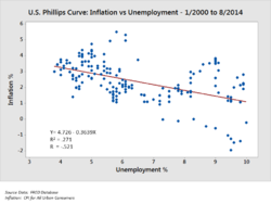
U.S. inflation and unemployment 1/2000 to 8/2014
However, in the 1990s in the US, it became increasingly clear that the NAIRU did not have a unique equilibrium and could change in unpredictable ways. In the late 1990s, the actual unemployment rate fell below 4% of the labor force, much lower than almost all estimates of the NAIRU. But inflation stayed very moderate rather than accelerating. So, just as the Phillips curve had become a subject of debate, so did the NAIRU.
Furthermore, the concept of rational expectations had become subject to much doubt when it became clear that the main assumption of models based on it was that there exists a single (unique) equilibrium in the economy that is set ahead of time, determined independently of demand conditions. The experience of the 1990s suggests that this assumption cannot be sustained.
Theoretical implications
To Milton Friedman there is a short-term correlation between inflation shocks and employment. When an inflationary surprise occurs, workers are fooled into accepting lower pay because they do not see the fall in real wages right away. Firms hire them because they see the inflation as allowing higher profits for given nominal wages. This is a movement along the Phillips curve as with change A. Eventually, workers discover that real wages have fallen, so they push for higher money wages. This causes the Phillips curve to shift upward and to the right, as with B. Some research underlines that some implicit and serious assumptions are actually in the background of the Friedmanian Phillips curve. This information asymmetry and a special pattern of flexibility of prices and wages are both necessary if one wants to maintain the mechanism told by Friedman. However, as it is argued, these presumptions remain completely unrevealed and theoretically ungrounded by Friedman.[30]
The last reflects inflationary expectations and the price/wage spiral. Supply shocks and changes in built-in inflation are the main factors shifting the short-run Phillips curve and changing the trade-off. In this theory, it is not only inflationary expectations that can cause stagflation. For example, the steep climb of oil prices during the 1970s could have this result.
Changes in built-in inflation follow the partial-adjustment logic behind most theories of the NAIRU:
Low unemployment encourages high inflation, as with the simple Phillips curve. But if unemployment stays low and inflation stays high for a long time, as in the late 1960s in the U.S., both inflationary expectations and the price/wage spiral accelerate. This shifts the short-run Phillips curve upward and rightward, so that more inflation is seen at any given unemployment rate. (This is with shift B in the diagram.)
High unemployment encourages low inflation, again as with a simple Phillips curve. But if unemployment stays high and inflation stays low for a long time, as in the early 1980s in the U.S., both inflationary expectations and the price/wage spiral slow. This shifts the short-run Phillips curve downward and leftward, so that less inflation is seen at each unemployment rate.
In between these two lies the NAIRU, where the Phillips curve does not have any inherent tendency to shift, so that the inflation rate is stable. However, there seems to be a range in the middle between "high" and "low" where built-in inflation stays stable. The ends of this "non-accelerating inflation range of unemployment rates" change over time.
12A. W. Phillips, ‘The Relation between Unemployment and the Rate of Change of Money Wage Rates in the United Kingdom 1861–1957’ (1958) 25 Economica 283, referring to unemployment and the "change of money wage rates". See (Fig 11, p. 297)
12Friedman, Milton (1968). "The Role of Monetary Policy". American Economic Review. 58 (1): 1–17. JSTOR1831652.
12Phelps, Edmund S. (1968). "Money-Wage Dynamics and Labor Market Equilibrium". Journal of Political Economy. 76 (S4): 678–711. doi:10.1086/259438. S2CID154427979.
12Phelps, Edmund S. (1967). "Phillips Curves, Expectations of Inflation and Optimal Unemployment over Time". Economica. 34 (135): 254–281. doi:10.2307/2552025. JSTOR2552025.
12Krugman, Paul R. (1995). Peddling prosperity: economic sense and nonsense in the age of diminished expectations. New York: W. W. Norton. p.43. ISBN978-0393312928.
↑Fisher, Irving (1973). "I discovered the Phillips curve: 'A statistical relation between unemployment and price changes'". Journal of Political Economy. 81 (2): 496–502. doi:10.1086/260048. JSTOR1830534. S2CID154013344. Reprinted from 1926 edition of International Labour Review.
↑Akerlof, George A.; Dickens, William T.; Perry, George L. (2000). "Near-Rational Wage and Price Setting and the Long-Run Phillips Curve". Brookings Papers on Economic Activity. 2000 (1): 1–60. CiteSeerX10.1.1.457.3874. doi:10.1353/eca.2000.0001. S2CID14610294.
↑Galbács, Peter (2015). The Theory of New Classical Macroeconomics. A Positive Critique. Contributions to Economics. Heidelberg/New York/Dordrecht/London: Springer. doi:10.1007/978-3-319-17578-2. ISBN978-3-319-17578-2.
This page is based on this Wikipedia article Text is available under the CC BY-SA 4.0 license; additional terms may apply. Images, videos and audio are available under their respective licenses.