Student's t-test

Student's t-test is a statistical test used to test whether the difference between the response of two groups is statistically significant or not. It is any statistical hypothesis test in which the test statistic follows a Student's t-distribution under the null hypothesis. It is most commonly applied when the test statistic would follow a normal distribution if the value of a scaling term in the test statistic were known (typically, the scaling term is unknown and is therefore a nuisance parameter). When the scaling term is estimated based on the data, the test statistic—under certain conditions—follows a Student's t distribution. The t-test's most common application is to test whether the means of two populations are significantly different. In many cases, a Z-test will yield very similar results to a t-test because the latter converges to the former as the size of the dataset increases.

History

William Sealy Gosset, who developed the "t-statistic" and published it under the pseudonym of "Student"

The term "t-statistic" is abbreviated from "hypothesis test statistic". ^[1] In statistics, the t-distribution was first derived as a posterior distribution in 1876 by Helmert ^{[2] [3] [4]} and Lüroth. ^{[5] [6] [7]} The t-distribution also appeared in a more general form as Pearson type  IV distribution in Karl Pearson's 1895 paper. ^[8] However, the t-distribution, also known as Student's t-distribution, gets its name from William Sealy Gosset, who first published it in English in 1908 in the scientific journal Biometrika using the pseudonym "Student" ^{[9] [10]} because his employer preferred staff to use pen names when publishing scientific papers. ^[11] Gosset worked at the Guinness Brewery in Dublin, Ireland, and was interested in the problems of small samples – for example, the chemical properties of barley with small sample sizes. Hence a second version of the etymology of the term Student is that Guinness did not want their competitors to know that they were using the t-test to determine the quality of raw material. Although it was William Gosset after whom the term "Student" is penned, it was actually through the work of Ronald Fisher that the distribution became well known as "Student's distribution" ^[12] and "Student's t-test".

Gosset devised the t-test as an economical way to monitor the quality of stout. The t-test work was submitted to and accepted in the journal Biometrika and published in 1908. ^[9]

Guinness had a policy of allowing technical staff leave for study (so-called "study leave"), which Gosset used during the first two terms of the 1906–1907 academic year in Professor Karl Pearson's Biometric Laboratory at University College London. ^[13] Gosset's identity was then known to fellow statisticians and to editor-in-chief Karl Pearson. ^[14]

Uses

One-sample t-test

A one-sample Student's t-test is a location test of whether the mean of a population has a value specified in a null hypothesis. In testing the null hypothesis that the population mean is equal to a specified value μ₀, one uses the statistic

${\displaystyle t={\frac {{\bar {x}}-\mu _{0}}{s/{\sqrt {n}}}},}$

where ${\displaystyle {\bar {x}}}$ is the sample mean, s is the sample standard deviation and n is the sample size. The degrees of freedom used in this test are n − 1. Although the parent population does not need to be normally distributed, the distribution of the population of sample means ${\displaystyle {\bar {x}}}$ is assumed to be normal.

By the central limit theorem, if the observations are independent and the second moment exists, then ${\displaystyle t}$ will be approximately normal ${\textstyle {\mathcal {N}}(0,1)}$.

Two-sample t-tests

Type I error of unpaired and paired two-sample t-tests as a function of the correlation. The simulated random numbers originate from a bivariate normal distribution with a variance of 1. The significance level is 5% and the number of cases is 60.

Power of unpaired and paired two-sample t-tests as a function of the correlation. The simulated random numbers originate from a bivariate normal distribution with a variance of 1 and a deviation of the expected value of 0.4. The significance level is 5% and the number of cases is 60.

A two-sample location test of the null hypothesis such that the means of two populations are equal. All such tests are usually called Student's t-tests, though strictly speaking that name should only be used if the variances of the two populations are also assumed to be equal; the form of the test used when this assumption is dropped is sometimes called Welch's t-test. These tests are often referred to as unpaired or independent samplest-tests, as they are typically applied when the statistical units underlying the two samples being compared are non-overlapping. ^[15]

Two-sample t-tests for a difference in means involve independent samples (unpaired samples) or paired samples. Paired t-tests are a form of blocking, and have greater power (probability of avoiding a type II error, also known as a false negative) than unpaired tests when the paired units are similar with respect to "noise factors" (see confounder) that are independent of membership in the two groups being compared. ^[16] In a different context, paired t-tests can be used to reduce the effects of confounding factors in an observational study.

Independent (unpaired) samples

The independent samples t-test is used when two separate sets of independent and identically distributed samples are obtained, and one variable from each of the two populations is compared. For example, suppose we are evaluating the effect of a medical treatment, and we enroll 100 subjects into our study, then randomly assign 50 subjects to the treatment group and 50 subjects to the control group. In this case, we have two independent samples and would use the unpaired form of the t-test.

Paired samples

Main article: Paired difference test

Paired samples t-tests typically consist of a sample of matched pairs of similar units, or one group of units that has been tested twice (a "repeated measures" t-test).

A typical example of the repeated measures t-test would be where subjects are tested prior to a treatment, say for high blood pressure, and the same subjects are tested again after treatment with a blood-pressure-lowering medication. By comparing the same patient's numbers before and after treatment, we are effectively using each patient as their own control. That way the correct rejection of the null hypothesis (here: of no difference made by the treatment) can become much more likely, with statistical power increasing simply because the random interpatient variation has now been eliminated. However, an increase of statistical power comes at a price: more tests are required, each subject having to be tested twice. Because half of the sample now depends on the other half, the paired version of Student's t-test has only ⁠n/2⁠ − 1 degrees of freedom (with n being the total number of observations). Pairs become individual test units, and the sample has to be doubled to achieve the same number of degrees of freedom. Normally, there are n − 1 degrees of freedom (with n being the total number of observations). ^[17]

A paired samples t-test based on a "matched-pairs sample" results from an unpaired sample that is subsequently used to form a paired sample, by using additional variables that were measured along with the variable of interest. ^[18] The matching is carried out by identifying pairs of values consisting of one observation from each of the two samples, where the pair is similar in terms of other measured variables. This approach is sometimes used in observational studies to reduce or eliminate the effects of confounding factors.

Paired samples t-tests are often referred to as "dependent samples t-tests".

Assumptions

^{[ dubious – discuss ]}

Most test statistics have the form t = Z/s, where Z and s are functions of the data.

Z may be sensitive to the alternative hypothesis (i.e., its magnitude tends to be larger when the alternative hypothesis is true), whereas s is a scaling parameter that allows the distribution of t to be determined.

As an example, in the one-sample t-test

${\displaystyle t={\frac {Z}{s}}={\frac {{\bar {X}}-\mu }{{\hat {\sigma }}/{\sqrt {n}}}},}$

where ${\displaystyle {\bar {X}}}$ is the sample mean from a sample X₁, X₂, …, X_n, of size n, s is the standard error of the mean, ${\displaystyle {\hat {\sigma }}={\sqrt {{\frac {1}{n-1}}\sum _{i}(X_{i}-{\bar {X}})^{2}}}}$ is the estimate of the standard deviation of the population, and μ is the population mean.

The assumptions underlying a t-test in the simplest form above are that:

• X follows a normal distribution with mean μ and variance σ²/n.
• s²(n − 1)/σ² follows a χ² distribution with n − 1 degrees of freedom. This assumption is met when the observations used for estimating s² come from a normal distribution (and i.i.d. for each group).
• Z and s are independent.

In the t-test comparing the means of two independent samples, the following assumptions should be met:

• The means of the two populations being compared should follow normal distributions. Under weak assumptions, this follows in large samples from the central limit theorem, even when the distribution of observations in each group is non-normal. ^[19]
• If using Student's original definition of the t-test, the two populations being compared should have the same variance (testable using F-test, Levene's test, Bartlett's test, or the Brown–Forsythe test; or assessable graphically using a Q–Q plot). If the sample sizes in the two groups being compared are equal, Student's original t-test is highly robust to the presence of unequal variances. ^[20] Welch's t-test is insensitive to equality of the variances regardless of whether the sample sizes are similar.
• The data used to carry out the test should either be sampled independently from the two populations being compared or be fully paired. This is in general not testable from the data, but if the data are known to be dependent (e.g. paired by test design), a dependent test has to be applied. For partially paired data, the classical independent t-tests may give invalid results as the test statistic might not follow a t distribution, while the dependent t-test is sub-optimal as it discards the unpaired data. ^[21]

Most two-sample t-tests are robust to all but large deviations from the assumptions. ^[22]

For exactness, the t-test and Z-test require normality of the sample means, and the t-test additionally requires that the sample variance follows a scaled χ² distribution, and that the sample mean and sample variance be statistically independent. Normality of the individual data values is not required if these conditions are met. By the central limit theorem, sample means of moderately large samples are often well-approximated by a normal distribution even if the data are not normally distributed. However, the sample size required for the sample means to converge to normality depends on the skewness of the distribution of the original data. The sample can vary from 30 to 100 or higher values depending on the skewness. ^{[23] [24]} F

For non-normal data, the distribution of the sample variance may deviate substantially from a χ² distribution.

However, if the sample size is large, Slutsky's theorem implies that the distribution of the sample variance has little effect on the distribution of the test statistic. That is, as sample size ${\displaystyle n}$ increases:

${\displaystyle {\sqrt {n}}({\bar {X}}-\mu )\xrightarrow {d} N(0,\sigma ^{2})}$ as per the Central limit theorem,

${\displaystyle s^{2}\xrightarrow {p} \sigma ^{2}}$ as per the law of large numbers,

${\displaystyle \therefore {\frac {{\sqrt {n}}({\bar {X}}-\mu )}{s}}\xrightarrow {d} N(0,1)}$.

Calculations

Explicit expressions that can be used to carry out various t-tests are given below. In each case, the formula for a test statistic that either exactly follows or closely approximates a t-distribution under the null hypothesis is given. Also, the appropriate degrees of freedom are given in each case. Each of these statistics can be used to carry out either a one-tailed or two-tailed test.

Once the t value and degrees of freedom are determined, a p-value can be found using a table of values from Student's t-distribution. If the calculated p-value is below the threshold chosen for statistical significance (usually the 0.10, the 0.05, or 0.01 level), then the null hypothesis is rejected in favor of the alternative hypothesis.

Slope of a regression line

Suppose one is fitting the model

${\displaystyle Y=\alpha +\beta x+\varepsilon ,}$

where x is known, α and β are unknown, ε is a normally distributed random variable with mean 0 and unknown variance σ², and Y is the outcome of interest. We want to test the null hypothesis that the slope β is equal to some specified value β₀ (often taken to be 0, in which case the null hypothesis is that x and y are uncorrelated).

Let

${\displaystyle {\begin{aligned}{\hat {\alpha }},{\hat {\beta }}&={\text{least-squares estimators}},\\SE_{\hat {\alpha }},SE_{\hat {\beta }}&={\text{the standard errors of least-squares estimators}}.\end{aligned}}}$

Then

${\displaystyle t_{\text{score}}={\frac {{\hat {\beta }}-\beta _{0}}{SE_{\hat {\beta }}}}\sim {\mathcal {T}}_{n-2}}$

has a t-distribution with n − 2 degrees of freedom if the null hypothesis is true. The standard error of the slope coefficient:

${\displaystyle SE_{\hat {\beta }}={\frac {\sqrt {\displaystyle {\frac {1}{n-2}}\sum _{i=1}^{n}(y_{i}-{\hat {y}}_{i})^{2}}}{\sqrt {\displaystyle \sum _{i=1}^{n}(x_{i}-{\bar {x}})^{2}}}}}$

can be written in terms of the residuals. Let

${\displaystyle {\begin{aligned}{\hat {\varepsilon }}_{i}&=y_{i}-{\hat {y}}_{i}=y_{i}-({\hat {\alpha }}+{\hat {\beta }}x_{i})={\text{residuals}}={\text{estimated errors}},\\{\text{SSR}}&=\sum _{i=1}^{n}{{\hat {\varepsilon }}_{i}}^{2}={\text{sum of squares of residuals}}.\end{aligned}}}$

Then t_score is given by

${\displaystyle t_{\text{score}}={\frac {({\hat {\beta }}-\beta _{0}){\sqrt {n-2}}}{\sqrt {\frac {SSR}{\sum _{i=1}^{n}(x_{i}-{\bar {x}})^{2}}}}}.}$

Another way to determine the t_score is

${\displaystyle t_{\text{score}}={\frac {r{\sqrt {n-2}}}{\sqrt {1-r^{2}}}},}$

where r is the Pearson correlation coefficient.

The t_{score, intercept} can be determined from the t_{score, slope}:

${\displaystyle t_{\text{score,intercept}}={\frac {\alpha }{\beta }}{\frac {t_{\text{score,slope}}}{\sqrt {s_{\text{x}}^{2}+{\bar {x}}^{2}}}},}$

where s_x² is the sample variance.

Independent two-sample t-test

Equal sample sizes and variance

Given two groups (1, 2), this test is only applicable when:

• the two sample sizes are equal,
• it can be assumed that the two distributions have the same variance.

Violations of these assumptions are discussed below.

The t statistic to test whether the means are different can be calculated as follows:

${\displaystyle t={\frac {{\bar {X}}_{1}-{\bar {X}}_{2}}{s_{p}{\sqrt {\frac {2}{n}}}}},}$

where

${\displaystyle s_{p}={\sqrt {\frac {s_{X_{1}}^{2}+s_{X_{2}}^{2}}{2}}}.}$

Here s_p is the pooled standard deviation for n = n₁ = n₂, and s ²
_X1 and s ²
_X2 are the unbiased estimators of the population variance. The denominator of t is the standard error of the difference between two means.

For significance testing, the degrees of freedom for this test is 2n − 2, where n is sample size.

Equal or unequal sample sizes, similar variances (⁠1/2⁠<⁠s_X1/s_X2⁠< 2)

This test is used only when it can be assumed that the two distributions have the same variance (when this assumption is violated, see below). The previous formulae are a special case of the formulae below, one recovers them when both samples are equal in size: n = n₁ = n₂.

The t statistic to test whether the means are different can be calculated as follows:

${\displaystyle t={\frac {{\bar {X}}_{1}-{\bar {X}}_{2}}{s_{p}\cdot {\sqrt {{\frac {1}{n_{1}}}+{\frac {1}{n_{2}}}}}}},}$

where

${\displaystyle s_{p}={\sqrt {\frac {(n_{1}-1)s_{X_{1}}^{2}+(n_{2}-1)s_{X_{2}}^{2}}{n_{1}+n_{2}-2}}}}$

is the pooled standard deviation of the two samples: it is defined in this way so that its square is an unbiased estimator of the common variance, whether or not the population means are the same. In these formulae, n_i − 1 is the number of degrees of freedom for each group, and the total sample size minus two (that is, n₁ + n₂ − 2) is the total number of degrees of freedom, which is used in significance testing.

The minimum detectable effect (MDE) is: ^[25]

${\displaystyle \delta \geq {\sqrt {\frac {2S_{p}^{2}}{n}}}(t_{1-\alpha ,\nu }+t_{1-\beta ,\nu })}$

Equal or unequal sample sizes, unequal variances (s_X1> 2s_X2 or s_X2> 2s_X1)

Main article: Welch's t-test

This test, also known as Welch's t-test, is used only when the two population variances are not assumed to be equal (the two sample sizes may or may not be equal) and hence must be estimated separately. The t statistic to test whether the population means are different is calculated as

${\displaystyle t={\frac {{\bar {X}}_{1}-{\bar {X}}_{2}}{s_{\bar {\Delta }}}},}$

where

${\displaystyle s_{\bar {\Delta }}={\sqrt {{\frac {s_{1}^{2}}{n_{1}}}+{\frac {s_{2}^{2}}{n_{2}}}}}.}$

Here s_i² is the unbiased estimator of the variance of each of the two samples with n_i = number of participants in group i (i = 1 or 2). In this case ${\displaystyle (s_{\bar {\Delta }})^{2}}$ is not a pooled variance. For use in significance testing, the distribution of the test statistic is approximated as an ordinary Student's t-distribution with the degrees of freedom calculated using

${\displaystyle {\text{d.f.}}={\frac {\left({\frac {s_{1}^{2}}{n_{1}}}+{\frac {s_{2}^{2}}{n_{2}}}\right)^{2}}{{\frac {(s_{1}^{2}/n_{1})^{2}}{n_{1}-1}}+{\frac {(s_{2}^{2}/n_{2})^{2}}{n_{2}-1}}}}.}$

This is known as the Welch–Satterthwaite equation. The true distribution of the test statistic actually depends (slightly) on the two unknown population variances (see Behrens–Fisher problem).

Exact method for unequal variances and sample sizes

The test ^[26] deals with the famous Behrens–Fisher problem, i.e., comparing the difference between the means of two normally distributed populations when the variances of the two populations are not assumed to be equal, based on two independent samples.

The test is developed as an exact test that allows for unequal sample sizes and unequal variances of two populations. The exact property still holds even with small extremely small and unbalanced sample sizes (e.g. ${\displaystyle n_{1}=5,n_{2}=50}$).

The statistic to test whether the means are different can be calculated as follows:

Let ${\displaystyle X=[X_{1},X_{2},\ldots ,X_{m}]^{T}}$ and ${\displaystyle Y=[Y_{1},Y_{2},\ldots ,Y_{n}]^{T}}$ be the i.i.d. sample vectors (${\displaystyle m\geq n}$) from ${\displaystyle N(\mu _{1},\sigma _{1}^{2})}$ and ${\displaystyle N(\mu _{2},\sigma _{2}^{2})}$ separately.

Let ${\displaystyle (P^{T})_{n\times n}}$ be an ${\displaystyle n\times n}$ orthogonal matrix whose elements of the first row are all ${\displaystyle 1/{\sqrt {n}}}$, similarly, let ${\displaystyle (Q^{T})_{n\times m}}$ be the first n rows of an ${\displaystyle m\times m}$ orthogonal matrix (whose elements of the first row are all ${\displaystyle 1/{\sqrt {m}}}$).

Then ${\displaystyle Z:=(Q^{T})_{n\times m}X/{\sqrt {m}}-(P^{T})_{n\times n}Y/{\sqrt {n}}}$ is an n-dimensional normal random vector.

${\displaystyle Z\sim N((\mu _{1}-\mu _{2},0,...,0)^{T},(\sigma _{1}^{2}/m+\sigma _{2}^{2}/n)I_{n}).}$

From the above distribution we see that

${\displaystyle Z_{1}={\bar {X}}-{\bar {Y}}={\frac {1}{m}}\sum _{i=1}^{m}X_{i}-{\frac {1}{n}}\sum _{j=1}^{n}Y_{j},}$

${\displaystyle Z_{1}-(\mu _{1}-\mu _{2})\sim N(0,\sigma _{1}^{2}/m+\sigma _{2}^{2}/n),}$

${\displaystyle {\frac {\sum _{i=2}^{n}Z_{i}^{2}}{n-1}}\sim {\frac {\chi _{n-1}^{2}}{n-1}}\times \left({\frac {\sigma _{1}^{2}}{m}}+{\frac {\sigma _{2}^{2}}{n}}\right)}$

${\displaystyle Z_{1}-(\mu _{1}-\mu _{2})\perp \sum _{i=2}^{n}Z_{i}^{2}.}$

${\displaystyle T_{e}:={\frac {Z_{1}-(\mu _{1}-\mu _{2})}{\sqrt {(\sum _{i=2}^{n}Z_{i}^{2})/(n-1)}}}\sim t_{n-1}.}$

Dependent t-test for paired samples

This test is used when the samples are dependent; that is, when there is only one sample that has been tested twice (repeated measures) or when there are two samples that have been matched or "paired". This is an example of a paired difference test. The t statistic is calculated as

${\displaystyle t={\frac {{\bar {X}}_{D}-\mu _{0}}{s_{D}/{\sqrt {n}}}},}$

where ${\displaystyle {\bar {X}}_{D}}$ and ${\displaystyle s_{D}}$ are the average and standard deviation of the differences between all pairs. The pairs are e.g. either one person's pre-test and post-test scores or between-pairs of persons matched into meaningful groups (for instance, drawn from the same family or age group: see table). The constant μ₀ is zero if we want to test whether the average of the difference is significantly different. The degree of freedom used is n − 1, where n represents the number of pairs.

Example of matched pairs Pair Name Age Test 1 John 35 250 1 Jane 36 340 2 Jimmy 22 460 2 Jessy 21 200

Example of repeated measures Number Name Test 1 Test 2 1 Mike 35% 67% 2 Melanie 50% 46% 3 Melissa 90% 86% 4 Mitchell 78% 91%

Worked examples

Let A₁ denote a set obtained by drawing a random sample of six measurements:

${\displaystyle A_{1}=\{30.02,\ 29.99,\ 30.11,\ 29.97,\ 30.01,\ 29.99\}}$

and let A₂ denote a second set obtained similarly:

${\displaystyle A_{2}=\{29.89,\ 29.93,\ 29.72,\ 29.98,\ 30.02,\ 29.98\}}$

These could be, for example, the weights of screws that were manufactured by two different machines.

We will carry out tests of the null hypothesis that the means of the populations from which the two samples were taken are equal.

The difference between the two sample means, each denoted by X_i, which appears in the numerator for all the two-sample testing approaches discussed above, is

${\displaystyle {\bar {X}}_{1}-{\bar {X}}_{2}=0.095.}$

The sample standard deviations for the two samples are approximately 0.05 and 0.11, respectively. For such small samples, a test of equality between the two population variances would not be very powerful. Since the sample sizes are equal, the two forms of the two-sample t-test will perform similarly in this example.

Unequal variances

If the approach for unequal variances (discussed above) is followed, the results are

${\displaystyle {\sqrt {{\frac {s_{1}^{2}}{n_{1}}}+{\frac {s_{2}^{2}}{n_{2}}}}}\approx 0.04849}$

and the degrees of freedom

${\displaystyle {\text{d.f.}}\approx 7.031.}$

The test statistic is approximately 1.959, which gives a two-tailed test p-value of 0.09077.

Equal variances

If the approach for equal variances (discussed above) is followed, the results are

${\displaystyle s_{p}\approx 0.08399}$

and the degrees of freedom

${\displaystyle {\text{d.f.}}=10.}$

The test statistic is approximately equal to 1.959, which gives a two-tailed p-value of 0.07857.

Related statistical tests

Alternatives to the t-test for location problems

The t-test provides an exact test for the equality of the means of two i.i.d. normal populations with unknown, but equal, variances. (Welch's t-test is a nearly exact test for the case where the data are normal but the variances may differ.) For moderately large samples and a one tailed test, the t-test is relatively robust to moderate violations of the normality assumption. ^[27] In large enough samples, the t-test asymptotically approaches the z-test, and becomes robust even to large deviations from normality. ^[19]

If the data are substantially non-normal and the sample size is small, the t-test can give misleading results. See Location test for Gaussian scale mixture distributions for some theory related to one particular family of non-normal distributions.

When the normality assumption does not hold, a non-parametric alternative to the t-test may have better statistical power. However, when data are non-normal with differing variances between groups, a t-test may have better type-1 error control than some non-parametric alternatives. ^[28] Furthermore, non-parametric methods, such as the Mann-Whitney U test discussed below, typically do not test for a difference of means, so should be used carefully if a difference of means is of primary scientific interest. ^[19] For example, Mann-Whitney U test will keep the type 1 error at the desired level alpha if both groups have the same distribution. It will also have power in detecting an alternative by which group B has the same distribution as A but after some shift by a constant (in which case there would indeed be a difference in the means of the two groups). However, there could be cases where group A and B will have different distributions but with the same means (such as two distributions, one with positive skewness and the other with a negative one, but shifted so to have the same means). In such cases, MW could have more than alpha level power in rejecting the Null hypothesis but attributing the interpretation of difference in means to such a result would be incorrect.

In the presence of an outlier, the t-test is not robust. For example, for two independent samples when the data distributions are asymmetric (that is, the distributions are skewed) or the distributions have large tails, then the Wilcoxon rank-sum test (also known as the Mann–Whitney U test) can have three to four times higher power than the t-test. ^{[27] [29] [30]} The nonparametric counterpart to the paired samples t-test is the Wilcoxon signed-rank test for paired samples. For a discussion on choosing between the t-test and nonparametric alternatives, see Lumley, et al. (2002). ^[19]

One-way analysis of variance (ANOVA) generalizes the two-sample t-test when the data belong to more than two groups.

A design which includes both paired observations and independent observations

When both paired observations and independent observations are present in the two sample design, assuming data are missing completely at random (MCAR), the paired observations or independent observations may be discarded in order to proceed with the standard tests above. Alternatively making use of all of the available data, assuming normality and MCAR, the generalized partially overlapping samples t-test could be used. ^[31]

Multivariate testing

Main article: Hotelling's T-squared distribution

A generalization of Student's t statistic, called Hotelling's t-squared statistic, allows for the testing of hypotheses on multiple (often correlated) measures within the same sample. For instance, a researcher might submit a number of subjects to a personality test consisting of multiple personality scales (e.g. the Minnesota Multiphasic Personality Inventory). Because measures of this type are usually positively correlated, it is not advisable to conduct separate univariate t-tests to test hypotheses, as these would neglect the covariance among measures and inflate the chance of falsely rejecting at least one hypothesis (Type I error). In this case a single multivariate test is preferable for hypothesis testing. Fisher's Method for combining multiple tests with alpha reduced for positive correlation among tests is one. Another is Hotelling's T² statistic follows a T² distribution. However, in practice the distribution is rarely used, since tabulated values for T² are hard to find. Usually, T² is converted instead to an F statistic.

For a one-sample multivariate test, the hypothesis is that the mean vector (μ) is equal to a given vector (μ₀). The test statistic is Hotelling's t²:

${\displaystyle t^{2}=n({\bar {\mathbf {x} }}-{{\boldsymbol {\mu }}_{0}})'{\mathbf {S} }^{-1}({\bar {\mathbf {x} }}-{{\boldsymbol {\mu }}_{0}})}$

where n is the sample size, x is the vector of column means and S is an m × m sample covariance matrix.

For a two-sample multivariate test, the hypothesis is that the mean vectors (μ₁, μ₂) of two samples are equal. The test statistic is Hotelling's two-sample t²:

${\displaystyle t^{2}={\frac {n_{1}n_{2}}{n_{1}+n_{2}}}\left({\bar {\mathbf {x} }}_{1}-{\bar {\mathbf {x} }}_{2}\right)'{\mathbf {S} _{\text{pooled}}}^{-1}\left({\bar {\mathbf {x} }}_{1}-{\bar {\mathbf {x} }}_{2}\right).}$

The two-sample t-test is a special case of simple linear regression

The two-sample t-test is a special case of simple linear regression as illustrated by the following example.

A clinical trial examines 6 patients given drug or placebo. Three (3) patients get 0 units of drug (the placebo group). Three (3) patients get 1 unit of drug (the active treatment group). At the end of treatment, the researchers measure the change from baseline in the number of words that each patient can recall in a memory test.

A table of the patients' word recall and drug dose values are shown below.

Patient	drug.dose	word.recall
1	0	1
2	0	2
3	0	3
4	1	5
5	1	6
6	1	7

Data and code are given for the analysis using the R programming language with the t.test and lmfunctions for the t-test and linear regression. Here are the same (fictitious) data above generated in R.

>word.recall.data=data.frame(drug.dose=c(0,0,0,1,1,1),word.recall=c(1,2,3,5,6,7))

Perform the t-test. Notice that the assumption of equal variance, var.equal=T, is required to make the analysis exactly equivalent to simple linear regression.

>with(word.recall.data,t.test(word.recall~drug.dose,var.equal=T))

Running the R code gives the following results.

• The mean word.recall in the 0 drug.dose group is 2.
• The mean word.recall in the 1 drug.dose group is 6.
• The difference between treatment groups in the mean word.recall is 6 – 2 = 4.
• The difference in word.recall between drug doses is significant (p=0.00805).

Perform a linear regression of the same data. Calculations may be performed using the R function lm() for a linear model.

>word.recall.data.lm=lm(word.recall~drug.dose,data=word.recall.data)>summary(word.recall.data.lm)

The linear regression provides a table of coefficients and p-values.

Coefficient	Estimate	Std. Error	t value	P-value
Intercept	2	0.5774	3.464	0.02572
drug.dose	4	0.8165	4.899	0.000805

The table of coefficients gives the following results.

• The estimate value of 2 for the intercept is the mean value of the word recall when the drug dose is 0.
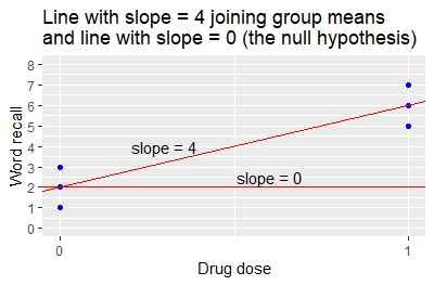
• The estimate value of 4 for the drug dose indicates that for a 1-unit change in drug dose (from 0 to 1) there is a 4-unit change in mean word recall (from 2 to 6). This is the slope of the line joining the two group means.
• The p-value that the slope of 4 is different from 0 is p = 0.00805.

The coefficients for the linear regression specify the slope and intercept of the line that joins the two group means, as illustrated in the graph. The intercept is 2 and the slope is 4.

Compare the result from the linear regression to the result from the t-test.

• From the t-test, the difference between the group means is 6-2=4.
• From the regression, the slope is also 4 indicating that a 1-unit change in drug dose (from 0 to 1) gives a 4-unit change in mean word recall (from 2 to 6).
• The t-test p-value for the difference in means, and the regression p-value for the slope, are both 0.00805. The methods give identical results.

This example shows that, for the special case of a simple linear regression where there is a single x-variable that has values 0 and 1, the t-test gives the same results as the linear regression. The relationship can also be shown algebraically.

Recognizing this relationship between the t-test and linear regression facilitates the use of multiple linear regression and multi-way analysis of variance. These alternatives to t-tests allow for the inclusion of additional explanatory variables that are associated with the response. Including such additional explanatory variables using regression or anova reduces the otherwise unexplained variance, and commonly yields greater power to detect differences than do two-sample t-tests.

Software implementations

Many spreadsheet programs and statistics packages, such as QtiPlot, LibreOffice Calc, Microsoft Excel, SAS, SPSS, Stata, DAP, gretl, R, Python, PSPP, Wolfram Mathematica, MATLAB and Minitab, include implementations of Student's t-test.

Language/Program	Function	Notes
Microsoft Excel pre 2010	TTEST(array1, array2, tails, type)	See
Microsoft Excel 2010 and later	T.TEST(array1, array2, tails, type)	See
Apple Numbers	TTEST(sample-1-values, sample-2-values, tails, test-type)	See
LibreOffice Calc	TTEST(Data1; Data2; Mode; Type)	See
Google Sheets	TTEST(range1, range2, tails, type)	See
Python	scipy.stats.ttest_ind(a, b, equal_var=True)	See
MATLAB	ttest(data1, data2)	See
Mathematica	TTest[{data1,data2}]	See
R	t.test(data1, data2, var.equal=TRUE)	See
SAS	PROC TTEST	See
Java	tTest(sample1, sample2)	See
Julia	EqualVarianceTTest(sample1, sample2)	See
Stata	ttest data1 == data2	See

See also

• Mathematics portal

• Conditional change model
• F-test  – Statistical hypothesis test, mostly using multiple restrictions
• Noncentral t-distribution in power analysis  – Probability distribution
• Student's t-statistic  – Ratio in statisticsPages displaying short descriptions of redirect targets
• Z-test  – Statistical test
• Mann–Whitney U test  – Nonparametric test of the null hypothesis
• Šidák correction for t-test  – Statistical method
• Welch's t-test  – Statistical test of whether two populations have equal means
• Analysis of variance  – Collection of statistical models (ANOVA)
• Confidence intervals for the mean of a normal distribution (also here)

References

1. The Microbiome in Health and Disease. Academic Press. 2020-05-29. p. 397. ISBN   978-0-12-820001-8.
2. Szabó, István (2003). "Systeme aus einer endlichen Anzahl starrer Körper". Einführung in die Technische Mechanik (in German). Springer Berlin Heidelberg. pp. 196–199. doi:10.1007/978-3-642-61925-0_16 (inactive 1 November 2024). ISBN   978-3-540-13293-6.
3. Schlyvitch, B. (October 1937). "Untersuchungen über den anastomotischen Kanal zwischen der Arteria coeliaca und mesenterica superior und damit in Zusammenhang stehende Fragen". Zeitschrift für Anatomie und Entwicklungsgeschichte (in German). 107 (6): 709–737. doi:10.1007/bf02118337. ISSN   0340-2061. S2CID   27311567.
4. Helmert (1876). "Die Genauigkeit der Formel von Peters zur Berechnung des wahrscheinlichen Beobachtungsfehlers directer Beobachtungen gleicher Genauigkeit". Astronomische Nachrichten (in German). 88 (8–9): 113–131. Bibcode:1876AN.....88..113H. doi:10.1002/asna.18760880802.
5. Lüroth, J. (1876). "Vergleichung von zwei Werthen des wahrscheinlichen Fehlers". Astronomische Nachrichten (in German). 87 (14): 209–220. Bibcode:1876AN.....87..209L. doi:10.1002/asna.18760871402.
6. Pfanzagl, J. (1996). "Studies in the history of probability and statistics XLIV. A forerunner of the t-distribution". Biometrika. 83 (4): 891–898. doi:10.1093/biomet/83.4.891. MR   1766040.
7. Sheynin, Oscar (1995). "Helmert's work in the theory of errors". Archive for History of Exact Sciences. 49 (1): 73–104. doi:10.1007/BF00374700. ISSN   0003-9519. S2CID   121241599.
8. Pearson, Karl (1895). "X. Contributions to the mathematical theory of evolution.—II. Skew variation in homogeneous material". Philosophical Transactions of the Royal Society of London A. 186: 343–414. Bibcode:1895RSPTA.186..343P. doi: 10.1098/rsta.1895.0010 .
9. Student (1908). "The Probable Error of a Mean" (PDF). Biometrika . 6 (1): 1–25. doi:10.1093/biomet/6.1.1. hdl:10338.dmlcz/143545 . Retrieved 24 July 2016.
10. "T Table".
11. Wendl, Michael C. (2016). "Pseudonymous fame". Science. 351 (6280): 1406. doi:10.1126/science.351.6280.1406. PMID   27013722.
12. Walpole, Ronald E. (2006). Probability & statistics for engineers & scientists. Myers, H. Raymond (7th ed.). New Delhi: Pearson. ISBN   81-7758-404-9. OCLC   818811849.
13. Raju, T. N. (2005). "William Sealy Gosset and William A. Silverman: Two 'Students' of Science". Pediatrics . 116 (3): 732–735. doi:10.1542/peds.2005-1134. PMID   16140715. S2CID   32745754.
14. Dodge, Yadolah (2008). The Concise Encyclopedia of Statistics. Springer Science & Business Media. pp. 234–235. ISBN   978-0-387-31742-7.
15. Fadem, Barbara (2008). High-Yield Behavioral Science. High-Yield Series. Hagerstown, MD: Lippincott Williams & Wilkins. ISBN   9781451130300.
16. Rice, John A. (2006). Mathematical Statistics and Data Analysis (3rd ed.). Duxbury Advanced.^{[ ISBN missing ]}
17. Weisstein, Eric. "Student's t-Distribution". mathworld.wolfram.com.
18. David, H. A.; Gunnink, Jason L. (1997). "The Paired t Test Under Artificial Pairing". The American Statistician. 51 (1): 9–12. doi:10.2307/2684684. JSTOR   2684684.
19. Lumley, Thomas; Diehr, Paula; Emerson, Scott; Chen, Lu (May 2002). "The Importance of the Normality Assumption in Large Public Health Data Sets". Annual Review of Public Health. 23 (1): 151–169. doi: 10.1146/annurev.publhealth.23.100901.140546 . ISSN   0163-7525. PMID   11910059.
20. Markowski, Carol A.; Markowski, Edward P. (1990). "Conditions for the Effectiveness of a Preliminary Test of Variance". The American Statistician. 44 (4): 322–326. doi:10.2307/2684360. JSTOR   2684360.
21. Guo, Beibei; Yuan, Ying (2017). "A comparative review of methods for comparing means using partially paired data". Statistical Methods in Medical Research. 26 (3): 1323–1340. doi:10.1177/0962280215577111. PMID   25834090. S2CID   46598415.
22. Bland, Martin (1995). An Introduction to Medical Statistics. Oxford University Press. p. 168. ISBN   978-0-19-262428-4.
23. "Central limit theorem and the normality assumption > Normality > Continuous distributions > Distribution > Statistical Reference Guide | Analyse-it® 6.15 documentation". analyse-it.com. Retrieved 2024-05-17.
24. DEMİR, Süleyman (2022-06-26). "Comparison of Normality Tests in Terms of Sample Sizes under Different Skewness and Kurtosis Coefficients". International Journal of Assessment Tools in Education. 9 (2): 397–409. doi:10.21449/ijate.1101295. ISSN   2148-7456.
25. Minimum Detectable Difference for Two-Sample t-Test for Means. Equation and example adapted from Zar, 1984
26. Wang, Chang; Jia, Jinzhu (2022). "Te Test: A New Non-asymptotic T-test for Behrens-Fisher Problems". arXiv: 2210.16473 [math.ST].
27. Sawilowsky, Shlomo S.; Blair, R. Clifford (1992). "A More Realistic Look at the Robustness and Type II Error Properties of the t Test to Departures From Population Normality". Psychological Bulletin. 111 (2): 352–360. doi:10.1037/0033-2909.111.2.352.
28. Zimmerman, Donald W. (January 1998). "Invalidation of Parametric and Nonparametric Statistical Tests by Concurrent Violation of Two Assumptions". The Journal of Experimental Education. 67 (1): 55–68. doi:10.1080/00220979809598344. ISSN   0022-0973.
29. Blair, R. Clifford; Higgins, James J. (1980). "A Comparison of the Power of Wilcoxon's Rank-Sum Statistic to That of Student's t Statistic Under Various Nonnormal Distributions". Journal of Educational Statistics. 5 (4): 309–335. doi:10.2307/1164905. JSTOR   1164905.
30. Fay, Michael P.; Proschan, Michael A. (2010). "Wilcoxon–Mann–Whitney or t-test? On assumptions for hypothesis tests and multiple interpretations of decision rules". Statistics Surveys. 4: 1–39. doi:10.1214/09-SS051. PMC   2857732 . PMID   20414472.
31. Derrick, B; Toher, D; White, P (2017). "How to compare the means of two samples that include paired observations and independent observations: A companion to Derrick, Russ, Toher and White (2017)" (PDF). The Quantitative Methods for Psychology. 13 (2): 120–126. doi: 10.20982/tqmp.13.2.p120 .

Sources

• O'Mahony, Michael (1986). Sensory Evaluation of Food: Statistical Methods and Procedures. CRC Press. p. 487. ISBN   0-82477337-3.
• Press, William H.; Teukolsky, Saul A.; Vetterling, William T.; Flannery, Brian P. (1992). Numerical Recipes in C: The Art of Scientific Computing. Cambridge University Press. p.  616. ISBN   0-521-43108-5.

Further reading

• Boneau, C. Alan (1960). "The effects of violations of assumptions underlying the t test". Psychological Bulletin. 57 (1): 49–64. doi:10.1037/h0041412. PMID   13802482.
• Edgell, Stephen E.; Noon, Sheila M. (1984). "Effect of violation of normality on the t test of the correlation coefficient". Psychological Bulletin. 95 (3): 576–583. doi:10.1037/0033-2909.95.3.576.

External links

• "Student test". Encyclopedia of Mathematics . EMS Press. 2001 [1994].
• Trochim, William M.K. "The T-Test", Research Methods Knowledge Base, conjoint.ly
• Econometrics lecture (topic: hypothesis testing) on YouTube by Mark Thoma